Chapter 2

Brushing Up on Math

In This Chapter

Reviewing basic algebra

Finding the love for trig

Calculating complex arithmetic

Recalling calculus

Rooting for polynomials

Can you believe it? A mathematics review chapter in a signals and systems book! Well, yes, you saw it coming. Mathematics plays a starring role in the study of signals and systems, which is basically a discipline of applied math.

In this chapter, I cover the mathematical concepts that you need for studying signals and systems, including specific aspects of algebra, trigonometry, complex arithmetic, calculus, and polynomial roots. So grab what you need from this chapter, and come back as necessary when you're trying to decipher the core concepts of signals and systems. If you need a more rigorous review of mathematical tools than what I provide here, check out Calculus For Dummies (Wiley) and other For Dummies resources available at www.dummies.com.

Revealing Unknowns with Algebra

Algebraic manipulation is at the core of many engineering calculations, especially in the study of signals and systems. After all, when three variables are at play, you can solve for any one by fixing the other two, using algebra. This is helpful because in design problems, you often need to meet some requirement but have one or more design values to choose. For the case of two design values, just pick a value for one and satisfy the requirement by solving for the remaining design value.

In the following sections, I review fundamental algebra concepts for two equations and two unknowns. I also cover partial fraction expansion (PFE), which is an algebraic technique for splitting up a ratio of polynomials into a sum of fractions, each having a denominator containing a single or repeated root.

Solving for two variables

To restart your algebraic manipulation engine, consider finding the values for two variables given two equations.

Example 2-1: A linear chirp signal involves changing the pitch, or frequency, of a single tone signal linearly with time. The instantaneous signal frequency is fi(t) = 2μt + f0 (Hz), where μ and f0 are constants. The units of fi(t) are hertz (Hz), or cycles per second. A design task is to produce a linear chirp signal from 200 Hz to 3,500 Hz over the time interval 0 ≤ t ≤ 10 s.

Notice that this problem requires you to solve for two unknowns. Here’s how to find the solutions:

1. Create two equations by using the start and stop time for the chirp as boundary conditions:

2. In the first equation, note that f0 = 200 Hz. In the second equation, 3,500 = 20μ + f0 = 20μ + 200.

3. Solve for μ:

Checking solutions with computer tools

A computer algebra system (CAS) can help you solve problems and check your work. One CAS option is the open-source software tool Maxima (see Chapter 1 for details).

Note: I use the GUI environment wxMaxima throughout this book for computer algebra-oriented calculations — problems that involve symbols and numbers.

Create this command line solution with wxMaxima:

In wxMaxima, each cell is an individual calculation. The first line of a cell is the input you type into Maxima; the second line is the output you get after using the key stroke Shift + Enter.

In solving for and , the input consists of two equations entered as a list followed by the variables to be solved for, which are also a list. A list is simply quantities placed between brackets and separated by commas, such as [mu, f0].

Exploring partial fraction expansion

Partial fraction expansion (PFE) techniques are important to the inverse Laplace transform (covered in Chapter 13) and the inverse z-transform (described in Chapter 14). These techniques make it possible to use a set of transform tables instead of contour integration from complex variable theory. With PFE, you split up a ratio of polynomials into a sum of fractions, each having a denominator containing a single or repeated root.

Consider the Nth-order polynomial:

And the Mth-order polynomial:

In the case of M < N, N(s)/D(s) is a proper rational function, meaning the degree of the numerator is less than the degree of the denominator. If you assume that pi, i = 1, . . . , N are distinct roots of D(s) — that is, no roots are repeated — then the PFE of N(s)/D(s) is

In the general case, again M < N, each of r roots of D(s) may have multiplicity , such that .

The PFE now takes the more complex form

When M ≥ N, you need to use long division to reduce the order of N(s) to be less than D(s) and then continue with the expansion. However, not taking this step to reduce the order of N(s) doesn’t prevent you from getting Ai values. But the values are incorrect, and you have no way of knowing this unless you recombine your expansion terms over a common denominator to see whether you return to the starting point.

With polynomial long division, your goal is

where is proper rational. Here’s how polynomial long division works:

Carrying out long division requires two steps. One is a setup, and the other is the long division itself, which repeats M – N + 1 times. Note that M – N long division brings numerator/denominator order parity, so you need to do one additional long division to make the numerator order one less than the denominator.

1. For the setup, multiply out the denominator into one big polynomial; for example, s(s – 2) = s2 – 2s.

2. Perform long division one time because :

3. Notice that the numerator order is reduced to M = 1 because the remainder is and , making

4. The roots of D(s) are 0 and 2, so the PFE of is

With the conversion from an improper rational function to a proper rational function now complete, you can move on to finding the expansion coefficients.

For the case of distinct roots, the formula for the coefficients is

When working with repeated roots, the formula is

Example 2-2: To find the expansion coefficients for , follow this process:

1. Verify that the function is proper rational.

Because 2 < 3, it’s proper rational.

2. Expand the formula:

3. One by one, solve for the coefficients:

4. Put the numerical coefficients in place to get the PFE representation:

5. Check your calculations with the Maxima function partfrac():

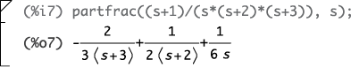
Note: Maxima chooses the expansion coefficient order, so you need to verify that the same terms are present in both solutions, independent of the order you chose for the hand calculation.

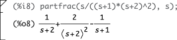
Example 2-3: Consider a partial fraction expansion for D(s) having one distinct root and a single root repeated, for a total of three roots. The function is proper rational (M = 1, N = 3), so use the repeated roots formulation of the PFE:

Because the first root is distinct, I made the connection that in the coefficient formulas.

Here’s how to determine the expansion coefficients:

1. Find the coefficients A1 and A22 by using the PFE coefficient formulas:

2. Find the coefficient A21.

The coefficient formula in this case involves taking a derivative of a ratio of polynomials. You can do this all right, but it’s tedious and error prone. For this type of problem, I prefer to find the coefficient by writing one equation to solve for the one unknown, A21 in this case. Choose a value for s where denominator terms are never 0. By choosing s = 1, you can work the algebra to solve for A21:

3. Put the numerical coefficients in place to establish the PFE representation:

4. Check your calculations with the Maxima function partfrac():

I explore the SciPy package signal and its functions residue and residuez in Chapters 15 and 14, respectively, as tools to numerically find the expansion coefficients.

Making Nice Signal Models with Trig Functions

When someone says the word trigonometry, what comes to mind? That ulcer you had freshman year, maybe? Okay, perhaps trig isn’t an exciting subject for you. Nevertheless, signal modeling and signal analysis using trig functions is a fact of life in electrical engineering.

That’s right; trigonometry is part of signal modeling (see Chapters 3 and 4), and trig functions are the basis of line spectra and Fourier series (Chapter 8), the Fourier transform (Chapter 9), and the discrete Fourier transform (Chapter 11). I know, there’s never a dull moment here; trig is the gig.

I explain how trig functions in complex arithmetic in the next section; but before we get into all of that, take a look at some of the most beloved trig identities in Table 2-1. Come back here when you need an identity or two as you work through trig functions.

Table 2-1 Useful Trig Identities

sinu = cos(u – π/2)	cosu = sin(u + π/2)
cos(u ± 2πk) = cosu, k = ± 1, ± 2, . . .	cos(–u) = cosu
sin(–u) = –sin(u)	sin2u + cos2u = 1
cos2u – sin2u = cos2u	2sinucosu = sin2u
sin(u ± v) = sinucosv ± cosusinv

These signal model examples can get you started with some common trig functions.

Example 2-4: A single continuous-time sinusoid takes the form x(t) = Acos(2πf0t + θ), –∞ < t < ∞, where A is the amplitude, f0 is the frequency in hertz, and θ is the phase in radians. If, say, θ = –π/2, then using the identity sinu = cos(u – π/2), you can write x(t) = Asin(2πf0t).

Example 2-5: Pressing a key on a telephone touchpad generates two tones. If you press 5, the row and column sinusoid frequencies are 770 Hz and 1,336 Hz, respectively. The signal you generate and hear is in this form:

x(t) = A{cos[2π(770)t] + cos[2π(1,336)t]}, Tstart ≤ t ≤ Tstop

Go ahead and press a key on a telephone right now and see whether you can discern two tones being played. This reveals a practical application of trig; it’s at work when you make a simple phone call! Trig and signal generation go hand in hand.

Manipulating Numbers: Essential Complex Arithmetic

Complex arithmetic is at the core of both analysis and design tasks performed by signals and systems engineers. Being able to manipulate complex numbers by using paper, pencil, and a pocket calculator on the fly is imperative. So I strongly suggest that you work the examples in this section on your pocket calculator.

Knowing how to use the tools available to you is also important. Using computer programs to manipulate complex numbers and check your answers is a part of everyday signals and systems work, so I give numerical examples in Python to back up hand-calculator calculations.

You need a scientific calculator to work complex arithmetic problems efficiently. Don’t expect Apple’s Siri to be there, spouting out answers for you. You need to get to know your scientific calculator — before you actually need it. So spend time digging into the details of how the calculator works, and practice! The payoff is quick calculations and peace of mind.

Believing in imaginary numbers

Imaginary numbers are indeed real, but they have a special multiplicative scale factor that makes them imaginary. The need for imaginary numbers comes about when you try to solve an equation involving the square root of a negative number. The scale factor represents the square root of –1 but is denoted with the letters i and j.

A complex number is composed of a real part x and or i times the imaginary part, y: z = x + jy, where .

Electrical engineers typically use j as the imaginary part scale factor because i usually denotes current. When viewed in the complex plane, the real part lies along the horizontal axis, and the imaginary part lies along the vertical or j axis. Therefore, a complex number is like a point (x, y) in a 2D Cartesian coordinate system.

As you may have heard in a physics and/or an analytic geometry course, the location of an object or point in two dimensions can be viewed as an order pair (x, y) and also as , where and are unit vectors pointing along the positive x- and y-axis, respectively. The same idea holds in the complex plane, but the operator rules are different. The imaginary part, y, is a real number just like the real part, x, is a real number. Also keep in mind that , so j · j = –1.

The rectangular (real/imaginary part) form of a complex number is z = (x, y) = x + jy. The corresponding polar form (magnitude and angle form) is z = (r, θ) = r · ejθ = |z|ejarg(z) = r∠θ, where, just like in 2D vector analysis, is the magnitude, and θ = arctan(y/x) is the angle in radians (arctan = tan–1). Voilà! I just described the rectangular-to-polar conversion operation. To get the angle in degrees from radians, you just need to convert, using the factor 180 degrees/π radians.

Finding the angle of a complex number by using arctan can be tough. The arctan function produces the proper angle only if the complex number lies in Quadrants I or IV. But arctan(y/x) can’t discern where the negative values occur in the ratio y/x, so you find complex numbers that lie in Quadrants II and III by using π + arctan(y/x).

If you’re using a calculator that supports complex number operations, use the built-in complex number capability. If you’re using a tool such as Python with PyLab, use abs(z) to find the magnitude and angle(z) or arctan2(y, x) to directly get the angle. See Examples 2-6 and 2-7 for details.

A polar-to-rectangular conversion takes you back to rectangular form: .

Example 2-6: Consider za = 3 + j4. Find za in polar form, following these steps:

1. Calculate the magnitude of za.

The magnitude is .

2. Find the angle of za.

Because 3 and 4 are both positive, you know that the point lies in Quadrant I. The angle of za is given by the arctan alone: radians.

Putting these two steps together gives you za=5ej0.9273, which is the polar form of za.

Check out a graphical depiction of resolving the proper quadrant for when using arctan in Figure 2-1.

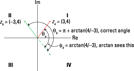
Figure 2-1: Finding the proper quadrant for the angles of complex numbers za and zb when using arctan.

Using Python with PyLab, you can convert the complex number to magnitude and angle:

In [28]: z_a = 3 + 4j

In [29]: abs(z_a)

Out[29]: 5.0

In [30]: angle(z_a) # angle in radians by default

Out[30]: 0.9272

In [31]: angle(z_a, deg=True) # gives angle in degrees

Out[31]: 53.130

Example 2-7: Test your ability to resolve the proper quadrant when using arctan by considering zb = –3 + j4. Find zb in polar form in two steps:

1. Calculate the magnitude of zb.

The magnitude of zb is .

2. Find the angle of zb.

Because 3 is negative and 4 is positive, you know that the point lies in Quadrant II. The angle of zb is given by radians.

Therefore, the polar form of is zb=5ej2.2143.

The details of the angle calculation are depicted in Figure 2-1. Using Python with PyLab, you can convert the complex number to magnitude and angle:

In [32]: z_b = -3 + 4j

In [33]: abs(z_b)

Out[33]: 5.0

In [34]: angle(z_b)

Out[34]: 2.2143

Example 2-8: Consider zc = 2ejπ/3. Find zc in rectangular coordinates in one step:

Looking at zc reveals that rc = 2 and θc = π/3, so .

Using Python, the calculation is direct:

In [41]: z_c = 2*exp(1j*pi/3.) # enter in polar form

In [42]: z_c

Out[42]: (1.0000+1.7321j)

Operating with the basics

The basic arithmetic operations with complex numbers are addition, subtraction, multiplication, and division. Addition and subtraction are easiest in rectangular form, and multiplication and division are easiest in polar form. Table 2-2 shows the formulas for the four operations, starting from z1 = x1 + jy1 and z2 = x2 + jy2.

Table 2-2 Basic Complex Math Operations

Operation	Formula
Add: z3 = z1 + z2	(x1 + x2) + j(y1 + y2)
Subtract: z3 = z1 – z2	(x1 – x2) + j(y1 – y2)
Multiply: z3 = z1z2 (polar form)	(x1x2 – y1y2) + j(x1y2 + y1x2)
Divide: z3 = z1/z2 (polar form)

Another basic operation is complex conjugation: when z = x + jy.

Note that z · z* = (x + jy)(x – jy) = x2 + y2 = |z|2.

At times, you may want to deal with only the real or imaginary part of an expression. The notation for the real part (real part operator) is Re{z} = Re{x + jy} = x. The notation for the imaginary part (imaginary part operator) is Im{z} = Im{x + jy} = y. As a simple example, .

Next, work through some calculations that utilize the basic complex math operations. Getting familiar with these types of calculations helps you prepare for more complicated topics in signals and systems.

Example 2-9: Let z1 = 1 + j7 and z2 = –4 – j9. The operations of Table 2-2 occur frequently, so it’s time to run some numbers for z1 + z2, z1z2, and z1/z2. Here’s how to work through the four calculations in sequence:

1. Find the sum, z1 + z2, following immediately from the formula of Table 2-2.

The real parts add and the imaginary parts add: z1 + z2 = [1 + (–4)] + j[7 + (–9)] = –3 – j2.

2. Work the multiplication result by using the polar form formula given in the multiplication row of Table 2-2.

Begin by first converting z1 and z2 to polar form (see Examples 2-6 and 2-7), and then multiply the magnitudes and add the angles to find the polar form of the answer. Finally, convert back to rectangular form:

3. Work the division, using the polar form formula of the division row of Table 2-2.

Start with the polar form answers from Step 2, divide the magnitudes and subtract the angles, and finally convert back to rectangular form:

4. Using Python with PyLab as a numerical tool, check your results:

In [57]: z_1 = 1 + 7j # define z1

In [58]: z_2 = -4 - 9j # define z2

In [59]: z_1 + z_2 # form the sum

Out[59]: (-3-2j)

In [60]: z_1*z_2 # form the product

Out[60]: (59-37j)

In [61]: z_1/z_2 # form the quotient

Out[61]: (-0.6907-0.1959j)

The Python results agree with the hand calculation. So pick up your calculator now and see whether you can get matching results.

Applying Euler’s identities

Euler’s formula is a useful mathematical result in signals and system analysis:

ejθ = cosθ + jsinθ

The formula is especially helpful when particular complex exponentials, where θ is a function of time, are used to develop the phasor addition formula (described in the next section). Given z = rejθ and Euler’s formula, the polar-to-rectangular conversion formula follows immediately, because z = rejθ = r(cosθ + jsinθ) = rcosθ + jrsinθ.

The inverse formula is perhaps even more useful:

In Part III of this book, I use both inverse formulas extensively, particularly to simplify expressions, demonstrating the importance of Euler’s identity in real-world signals and systems work. As a quick example of the formula’s practical application, consider factoring in the following to form a cosine:

Applying the phasor addition formula

When sinusoidal signals of like frequency ω0 are added together (superimposed), the result is a single sinusoidal signal having composite amplitude A and phase ϕ. In mathematical terms, given N sinusoidal functions (signals) each of identical frequency ω0, you can show that the sum

where, on the right side, the composite amplitude A and phase ϕ is related to the amplitude Ak and phase ϕk of each term through the summation.

Example 2-10: Given , find the composite signal . Follow these steps to get A and ϕ:

1. Rewrite the sine term as a cosine, so all terms in the sum fit the phasor addition formula mathematical form.

Using the Row 1/Column 1 trig identity of Table 2-1, .

2. Identify the magnitude and angles Akejϕk, k = 1, 2, two terms in the problem statement:

3. Add the two complex numbers that are in polar form.

4. Check the calculation on your calculator and then work the calculation in Python, as shown here:

In [115]: A_phi=4*exp(1j*pi/4.) + 15*exp(-1j*pi/2.)

In [117]: (abs(A_phi), angle(A_phi)) # polar form

Out[117]: (12.4959, -1.3425)

5. You find Aejϕ in Step 3; write out the final form by putting the magnitude in front of the cosine and entering the angle inside the argument of the cosine:

x(t) = 12.4959cos(ω0t – 1.3425)

---

---

Catching Up with Calculus

Single variable integration and differentiation are main calculus topics at play in signals and systems work. In this section, I provide a table of differentiation properties and a short table of indefinite and definite integrals. The tables are for quick reference as the need arises. I also point out simple optimization theory, including min and max and efficient numerical techniques.

And lest you think I may have completely spaced the importance of geometric series formulas, don’t worry! Formulas for finite and infinite geometric series are available in this section, too, so you can check back here if needed when you read Chapters 6, 11, and 14 on discrete-time signals and systems. I also describe tools for polynomial root finding in this section.

Differentiation

Finding the derivative of function is part of the core material in a calculus course. And being able to differentiate simple functions is essential to signals and systems analysis. This section reviews the fundamentals of differentiation and provides a table of key differentiation formulas.

The derivative of an equation is the slope at any point where the equation is evaluated. Formally, the function f(x) has derivative f'(x), at the point x if the limit exists.

If you need help when working problems where differentiation is involved, reference the differentiation formulas in Table 2-3. In this table, assume a is a constant and both u and v are possibly functions of x.

Table 2-3 Differentiation Formulas

Example 2-11: Given , find . To solve, use the formulas in Table 2-3:

You can also use the CAS Maxima to check this differentiation.

Integration

What differentiation does, integration undoes. In mathematical terms, the integral of the function f(x) is known as the antiderivative. The good news about signals and systems work is that although integration is present in the associated problem solving, you can use integration tables for both indefinite and definite integrals.

Indefinite integrals are the antiderivatives. So when I write

I’m saying that

In Table 2-4, I provide a collection of indefinite integrals that are useful for signals and systems work. In this table, assume a is a constant.

Table 2-4 Indefinite Integrals

Example 2-12: To see how numerical integration can be put into motion on a problem with known solution, find the integral of te–5t on the interval [0, 4] by using the Row 2/Column 2 entry of Table 2-4:

You can also use the CAS Maxima to check this integration.

Definite integrals, also known as integrals with fixed limits, are important in the study of signals and systems. Table 2-5 is a collection of useful definite integrals. In this table, assume a is a constant.

Table 2-5 Definite Integrals

When closed-form integration isn't workable — that is, if the integral isn't available in a table — you need to use numerical integration. By closed-form, I mean the solution can be written in terms of a small number of well-known functions. Tools such as Python and the integrate module of SciPy provide a collection of numerical integration routines. I use the function quad in Example 2-13.

Numerical integration saves you the trouble of an extensive search for a closed-form integral, and it may be your only option in some cases. But use numerical integration with care to ensure convergence to the proper solution.

Example 2-13: To gain confidence in the use of numerical integration, I repeat the integration of Example 2-12, using Python and the function quad from the SciPy module integrate:

In [90]: from scipy.integrate import quad

In [91]: def my_inte(t): # integrand function

    ...: return t*exp(-5*t)

In [92]: quad(my_inte,0,4) # integrate from 0 to 4

Out[92]: (0.03999999826863095, 7.91215216153553e-14)

In [93]: (1 - 21*exp(-20))/25.

Out[93]: 0.03999999826863096

The calculation requires a Python function, Line [91], to first represent the integrand. Second, you call quad with the integrand function name followed by the lower and upper limits. The function returns the integral and the absolute error (see Line [92]). Comparing Line [92] with the known closed-form solution of Line [93] reveals very close agreement.

System performance

When you design a system, you need to maximize, minimize, or find critical values of performance functions. A performance function, such as a time-domain or frequency-domain response, provides a means to demonstrate that your design meets requirements set by your customer. Calculus and numerical methods based on calculus can help.

Elementary calculus reveals that function f(x) is a maximum where the derivative is 0, as long as the function isn’t passing through an inflection point. So if the solution to is x0, does x0 correspond to a maximum or minimum? To find out, check the sign of the second derivative at x0. If , then x0 corresponds to a minimum. If , then x0 corresponds to a maximum.

Example 2-14: To minimize the quadratic function f(x) = x2 + 10x + 20, use this two-step process:

1. Take the derivative of f(x) and set the result equal to 0:

2. See whether the point corresponds to a maximum or minimum. Take the second derivative and check the sign at x0:

Example 2-15: More often than not, the performance function is nontrivial, meaning a pure calculus-based solution involves some work. Consider the step response waveform (see Chapter 13). A plot of this function is given in Figure 2-2.

This function rises up from 0 to 1 as t increases from 0 to infinity but with a small amount of overshoot, which means the function exceeds 1 before settling back to 1.

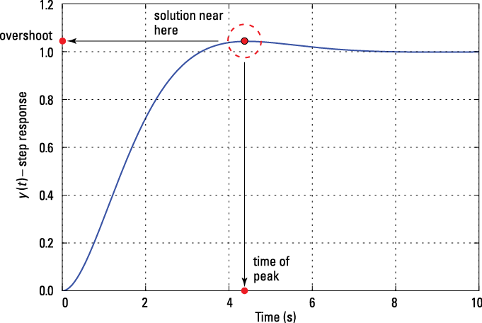
Figure 2-2: Plot of the step response y(t), showing the approximate location of the peak overshoot.

Suppose the overshoot value and the corresponding time are both needed for system performance assessment. You can find a numerical solution quickly by first filling an array with closely spaced values of y(t) over 2 to 6 s. Use max to get the maximum value on this interval, and then use find to find the array index where the maximum occurs. Finally, plug the index into the t array to reveal the time of the peak.

In [120]: t = arange(2,6,.001) # small time step

In [121]: y = 1-(exp(-t/sqrt(2))

*(sin(t/sqrt(2))+cos(t/sqrt(2))))

In [122]: max_y = max(y) # obtain peak numerically

In [123]: find(y == max_y) # find peak index

Out[123]: array([2443], dtype=int64) # at index 2443

In [124]: t_max = t[2443] # plug index into t array

In [125]: (max_y,t_max) # display results

Out[125]: (1.0432, 4.4429) # (overshoot, time in s)

The peak overshoot in this case is 1.0432, or about 4.3 percent, and it’s located at 4.44 s.

Geometric series

In the study of discrete-time signals and systems (covered in Chapters 6, 7, 11, 12, and 14), you frequently encounter geometric series — finite and infinite. For example, in Chapter 6, both forms arise in impulse response calculations, and in Chapters 11 and 14, where the discrete Fourier transform and z-transforms are studied, both forms are again essential for developing transform pairs.

The finite geometric series takes the following form, where a is a constant:

The infinite series takes this form:

Table 2-6 provides a short table of geometric series sums.

Table 2-6 Series Sum Formulas

Sum	Condition
	none
	none
	none
	|a| < 1
	|a| < 1

Example 2-16: To sum the series , follow this three-step process. Note: Table 2-6 doesn’t contain an exact fit for this summation, so you need to do some improvising.

1. Introduce a variable change to transform the sum to the standard form.

Let m = n – 5. Then, in the present sum, replace n with m + 5.

2. Transform the sum limits, too:

and

3. Put Steps 1 and 2 together in the original sum:

Finding Polynomial Roots

To perform stability analysis of systems (covered in Chapters 13 and 14), you need to be able to find the roots — values of the independent variable where the polynomial is 0 — of a polynomial of degree 2 and higher. The quadratic formula works for the second-order case, but numerical root finding is the best option for higher-order polynomials.

Numerical solving routines within Python and PyLab make calculating numerical roots a snap. Similar routines are available in other tool sets.

The problem here is to find the roots of the Nth-degree polynomial: .

The function pN = roots(AN) returns the polynomial roots into array pN given the coefficients aN, aN–1, … , a1, a0 are contained in the array AN.

A special Nth-degree polynomial that occurs in discrete-time systems modeling is P(s) = sN – 1. Yes, you can use roots for this polynomial, but an analytical solution, known as the roots of unity, is readily available. To solve, set P(s) = 0, so . The roots are

because

The roots are located in the complex plane equally spaced around the unit circle, at separation angle 2π/N.

A variation on the original polynomial is P1(s) = sN – aN. The N roots in this case take the same angle values but have magnitude a.