
Chapter 6
Exposimetry – Measurements of the
Ambient RF Electromagnetic Fields1
6.1. Introduction
Any moving electric charge produces an electromagnetic radiation which is propagated in space. This property is at the base of the production of electromagnetic radiations used in the devices of radio, television, telecommunication, heating by microwaves, emission radar. Consequently, any system fed in electricity or with stronger reason containing an aerial element emits an electromagnetic radiation or generates an electric and/or magnetic field in its close or even distant vicinity, that we will characterize in this article using the generic term of RF electromagnetic field. Two concerns emerge from this electromagnetic presence:
– one relates to the electronic systems and thus electromagnetic compatibility (CEM);
– the other is man, as a user, patient and human exposure to the electromagnetic fields induced by non-ionizing radiations (NIR). This last concern comes under the field of hygiene and safety.
This chapter dedicated to the measurement of the RF electromagnetic fields, in the frequency band concerned with non-ionizing radiations, relates to this last aspect exclusively. Even if it is a question of quantifying the same physical sizes, the differences of objectives, protocols, standardization and regulation and reference frame, measuring apparatus ensure that each concern preserves its own constraints and its characteristics and must be treated separately.
In order to bring reliable elements of appreciation to the medical persons in charge, the first element consists of quantifying, by measurement, the relevant sizes characterizing the exposure of the man. The object of this article is to describe “the good” practices of laboratories.
6.2. Definitions
They are general standards of physics applied to the specific character of the effects of the fields on the man:
– Basic restrictions: restrictions on the effects of exposure are based on established health effects and are called basic restrictions, current density, SAR and power density are the physical quantities used to specify these basic restrictions.
– Current density: current flowing through a unit of area perpendicular to the current flow in a conducting volume like the human body or part of this last. It is expressed in ampere per square meter (A/m2).
– Electromagnetic fields: in this chapter this expression includes/understands all the fields which are electric, magnetic or components of an electromagnetic wave, including the static fields, on the entire frequency band between 0 Hz and 300 GHz. These fields are likely to interact, in one way or another, with the living organisms (i.e. humans) subjected to their presence.
– Biological effect: reaction of the organism in response to an external factor and may or may not have a consequence on health.
– Dosimetry: using the intermediary of the SAR, quantifies the exposure to the electromagnetic fields of humans, animals or live cells.
– Effective values: values of the fields according to the equation:
![]()
where v (T) is the variation of the electric field or the magnetic field according to time and T is the period. It is defined mathematically as the effective value of the squares of the instantaneous values of the signal.
In EMC, the peak values, quasi-peak and average are preferred. In NIR, it is usual, for the continuous emissions, to give the fields in RMS values. However, for the pulsated sources, the fields are often expressed in peak values. Thus the RMS value is very often quasi-zero.
– Electric field intensity: value of the module of the electric field E, expressed in volt per meter (V/m).
– Electromagnetic compatibility (EMC): aptitude of a device, an apparatus or a system to functioned in its electromagnetic environment in a satisfactory way and without producing intolerable electromagnetic disturbances for all that is in this environment.
– Energy of the photons or quantum energy of a wave: product of the Planck's constant (![]() 34 J-s) by the frequency v expressed in hertz. The quantum energy hv, expressed in electron-volts, is relatively weak in the spectral field concerned, thus, the electromagnetic fields of 0 Hz to 300 GHz are often indicated by the expression “non-ionizing radiations or NIR”.
34 J-s) by the frequency v expressed in hertz. The quantum energy hv, expressed in electron-volts, is relatively weak in the spectral field concerned, thus, the electromagnetic fields of 0 Hz to 300 GHz are often indicated by the expression “non-ionizing radiations or NIR”.
– Evaluation of uncertainties of measurements of type a: evaluation of uncertainties by statistical analysis of the series of observation.
– Evaluation of uncertainties of measurements of type b: evaluation of uncertainties by means other than the statistical analysis of the series of observation.
– Exposimetry: measurements of electromagnetic field in the ambient environment.
– Far-field (zone of Fraunhofer): zone far away from the radiant structure of at least 1.6 times the wavelength; in this zone, the relations between electric field E, magnetic field H and density of density surface power S are clearly defined and the simple knowledge of a size makes it possible to determine the two others. The intensity of the wave varies in a way inversely proportional to the square of the distance and the modules of E and H are connected between them by the relation E/H = 377 ohms.
– Flux magnetic density or magnetic induction (B): is a vector quantity equivalent to the magnetic field in the air and biological environments. It is expressed in Tesla (T) with the following equivalence relations: ![]() 7 T. Gauss (G) although non-legal unit can still be met (1 μT = 10 MG).
7 T. Gauss (G) although non-legal unit can still be met (1 μT = 10 MG).
– Frequencies and wavelengths: the frequency is the number of vibrations or oscillations per unit of time in a periodic phenomenon. The majority of the fields vary sinusoidally at a frequency v, expressed in Hz, KHz, MHz or GHz. In a given medium, characterized by its permittivity ε and its permeability μ, the electromagnetic waves are propagated at a speed which is equal at the speed of light c in the vacuum and also practically in the air. The wavelength λ is related to the frequency by the relation: λ= v/c.
– Heating effect: biological effect which results in an increase in the temperature.
– Leakage level (in microwave): density of power in any point accessible located at a distance from at least 5 cm (“2 inches”) from a microwave apparatus. It is expressed in W/m2 or more practically in mW/cm2.
– Levels of reference: the reference levels are obtained from the basic restrictions by mathematical modeling and by extrapolation from the results of laboratory experiments; the levels of reference are expressed in the form of an electric field, a magnetic field or a density of power.
– Magnetic field strength: value of the module of the magnetic field H, it is expressed in ampere per meter (A/m).
– Magnetic field: involving the vector field of the magnetic forces of attraction or repulsion, due to the presence of an electrical current from the movement of charged particles. Its intensity is expressed in ampere per meter (A/m).
– Medical effect: biological effect having an effect on health
– Near-field (Fresnel zone): zone close to the radiant structure where the electromagnetic wave “is not formed”, it does not have the characteristics of wave planes and the electric and magnetic fields strongly vary from one point to another. E and H are not correlated and must be measured independently. In this zone, the electric and magnetic fields vary according to the place.
– Non-ionizing radiations (NIR): non-ionizing radiations are radiations whose energies are insufficient to ionize an atom, i.e. unable to tear off an electron with the matter.
– Polarization: orientation of the plan containing the electric vector field E and the direction of propagation wave:
- if the plan turns, it is known as revolving of elliptic-type, or circular according to the curve followed by the end of the electric vector field according to time;
- if this plan is fixed, polarization is known as linear of vertical-type if the vector E is vertical, and of horizontal-type if the vector E is horizontal.
– Power transported by a wave: the plane waves transport energy which is propagated parallel to the wave plane. The power is the energy delivered per second by a radiant system, it is expressed in Watt (W).
– Attention principle: even in the absence of scientific bases on effects proven on health, it is necessary to be respectful concerns of the public (for example, the principle of attention applies to the basic stations installed by the operators of mobile telephony).
– Precaution principle: principles such as the absence of certainty, taking into account the scientific and technical training of the moment, joining a great complexity, should not delay the action. This principle, by adopting effective and proportioned measurements, aims to prevent a risk of serious and irreversible damage, attenuating or limiting its consequences, at an economically acceptable cost, from the point of view of durable development (Tanzi, 2006).
– Specific absorption: is the absorbed energy per unit of biological tissue mass, expressed in joule per kilogram (J/kg).
– Specific absorption rate (SAR): expressed in Watt per kilogram, represents absorbed RF power per mass unit of a biological tissue, exposed to an electric field E (in V/m), and characterized by its electric conductivity σ (in S/m and its density of mass ρ (in kg/m3)
![]()
– Surface power density S or Poynting vector: the Poynting vector represents the density of the wave power, i.e. the power per unit of area. It is thus the quotient of the incidental power radiated by the surface perpendicular to the propagation direction. The density of power is expressed in Watt per square meter (W/m2) or more practically in mW/cm2 with 1 W/m2 = 0.1 mW/cm2.
In far-field, the intensity of the electric field (E), and the intensity of the magnetic field (H) are bound by the impedance of wave in free space (377 ohms):
![]()
where E and H are expressed in V/m and A/m and S in W/m2.
– Widened uncertainty: it defines an interval around a result of measurement, which we can expect that it includes/understands a high fraction of the distribution of the values which could reasonably be allotted to measurement.
6.3. Interactions of the electromagnetic fields with biological tissues and medical risks
6.3.1. What are the effects of the electromagnetic fields and waves on human health?
This is a constant question which is not ready to die out if we judge from the great number of scientific publications, television broadcasts and press articles devoted to this topic. This concern is increased besides by the constant increase in the population concerned:
– on the one hand, in the domestic field, with the high voltage lines, the microwave ovens, the induction plates and especially the radiotelephones;
– on the other hand, in the professional field with the installations of welding, induction or dielectric effect heater, the display screens of computers, telecommunications, the radars, etc.
For strong exposures, significantly higher than the recommended exposure limit values, hyperthermia partial or generalized of the human body, consecutive with these exposures, must be regarded as a very rare accident. Strict application of the standards and the limiting values should ensure that such exposures never take place. On the other hand, which makes debate, they are actually the exposures to weak fields whose intensities respect the limiting values of the current standards and for which various effects regularly advance from the simple nuisance to severe pathologies. We speak then about no thermal or specific effects.
At all events and in order to bring reliable elements of appreciation to the medical persons in charge, the first element of the answer consists of quantifying by measurement the relevant physical quantities characterizing the human exposure. It is a question of specifying the medical risk which the electromagnetic fields present in a field where knowledge still is not completely stabilized. Stock also, can be taken on current knowledge while being pressed on recent documents which one can find in the following references (www.who.int;www.sante-radiofrequences.org).
6.3.2. Duality wave-photon: remarks on activation energies
The photon is the elementary particle which transmits the electromagnetic interactions. By the duality wave-particle, the wave can be seen like a beam of photons. The energy of the photon is equal to the product of the Planck's constant h and the vibration frequency v of associated electromagnetic field: E = hv. Thus the electromagnetic waves of increasingly high frequencies or increasingly short wavelengths correspond to photons of an increasingly large energy. The photon does not carry an electric charge; it has zero mass and moves at the speed of light.
When a wave (or a particle) interacts with materials (solid, liquid or soft), its energy of activation has to be taken into account. Typically a binding energy of the atoms of a solid is about 10 eV. To break a connection between atoms, the incident particle (wave) must at least have this energy. However, as shown in Table 6.1, energies of the electromagnetic fields are much weaker. For example, to 1 GHz, energy is 4 μeV and thus, of course, far too weak to involve a displacement of atoms.
In the same way, to involve potential ionizations of materials energies must be about 1 eV. This is too very far from energies of RF waves, and we can thus only refute the possibility of material ionization (alive or not) interacting with RF waves.
In a stable state, any material is subjected from its temperature in a state of fluctuation known as being the Brownian movement or thermal noise and whose characteristic is kBT. kB is the constant of Boltzman, 86 μeV per K, and T the temperature in Kelvin. To 300 K, the fluctuation energy is 26 meV. As long as the activation energy brought by a wave remains much lower than 26 meV, there are no effects on the fluctuations induced by the Brownian movement and thus on the total behavior of materials and biological tissues. Consequently, there would be no possible biological effects for waves having energies significantly lower than 26 meV (i.e. in all the ranges of the radio frequencies from hertz to terahertz).
The photon returning in the matter interacts with it and is absorbed. This interaction with the matter, which is more or less strong according to its structure, causes it to stop in the matter. At the end of the course, it completely loses its energy in thermal form: very locally, hot nanoscopic zones are produced. With strong photon numbers, these hot nanoscopic zones can involve a significant heating of the irradiated matter.
The biological system is a complex system and balance, even a weak disturbance can, perhaps, involve an imbalance of the irradiated system. The effect brought by photons, or of an electromagnetic wave, on a biological system cannot be simply explained by considering only the interactions between photons and molecules. All the system balances must be considered.
6.3.3. RF fields are non-ionizing
The electromagnetic fields of the field of the non-ionizing radiations do not utilize mechanisms of quantum interaction contrary to the high part of the electromagnetic spectrum. Without entering a discussion on the possible risks of the low part of the electromagnetic spectrum, it is fundamental to reaffirm that the interaction-type with quantum transfer of energy cannot theoretically occur, which creates an essential difference with the high part of the electromagnetic spectrum (X and γ at the origin of molecular ionizations).
Mechanisms of interaction, devastators for the exposed medium, such as the effect Compton, the creation of electron-positron pairs, the photoelectric effect, etc. cannot appear which prohibits the transposition to these fields of knowledge and the step specific to the ionizing radiations. In other words, this weakness of equivalent energy certainly makes it possible to exclude the considered fields from the field of “poisons” with strong influence, without freeing them from harmful effects on health.
However, that does not prevent other mechanisms from occurring. The presence, in any biological environment, of ions, ferromagnetic substances, cells with an electric behavior, mediums having some dielectric properties involves and explains creation, in these mediums, of induced currents, localized or generalized heating, potential differences, etc. These mechanisms are well known and have as names: forces of Lorentz, dielectric absorption, Hall effect, Zeeman effect, etc.
They can be applied to the three families of fields, namely static magnetic fields, electric fields and extremely low frequency (ELF) magnetic fields and electromagnetic fields with radio frequencies and ultra high frequencies. The produced effects depend, on the one hand, on the characteristics of the incidental field (natural electric and/or magnetic, frequency, continuous or pulsated mode, modulation, etc.) and, on the other hand, on the characteristics of the exposed biological environment (dimensions, electric permittivity, magnetic permeability, etc.).
6.3.4. Biological effects of the electromagnetic field
As the human body is surrounded electromagnetic waves, and is composed of biological tissues it is useful to know the effects of waves RF on biological materials. If the material in interaction with the incident waves is a biological tissue, we have the same basic phenomena of interaction as with all other materials, except that the structure of a biological material is much more complex than a crystalline, polycrystalline or amorphous material.
The most commonly known effect is of thermal-type. It corresponds to the accumulation of thermal form energy in biologic tissues. For frequencies higher than 10 kHz, the SAR is the fundamental physical quantity which makes it possible to determine derived limit values, which are expressed in electric field intensity or surface power density. The majority of the experiments showed this heating effect when the SAR is higher than 4 W/kg, that is to say 10 times the exposure limit value of 0.4 W/kg (Table 6.1).
A strong over-exposure (>> 4 W/kg) led to excessive heating accidents with perception of heat, release of cephalgias, sometimes of neuropathy of the exposed zones, appearance of surface or deep burns. The same mechanism can certainly explain the increase in the permeability of the hemato-encephalic barrier, due to an increase in the cerebral temperature, as well as the appearance of cataracts. This excessive heating is theoretically possible but seldom reported because the exposed individuals quickly experience a feeling of heat and move away from the source by reflex of self-defense.
Effects of a different nature, nonrelated to a direct heating effect, are also recognized: the magnetohydrodynamic effect in the aorta explaining the modifications of the electrocardiogram, the disturbances of the orientation system of pigeons, bees, etc., the reduction in enzymatic activity, the cardiac risk of fibrillation to very strong exposure, the reduction in melatonin concentration likely to be implied as increasing the risk of breast cancer in relation to an electromagnetic exposure.
Moreover, the experiments highlighted that the combination of a static magnetic field and a magnetic field oscillating at a low frequency has an influence on the biological systems, without it still being possible to specify the methods of them.
Many other effects, which are not understandable by the traditional mechanisms, were shown on low levels of fields. The bibliography is rich with effects proven or not, on subcellular and cellular levels, membranes, growth of cells and their proliferation, level of a body or a system, the liver, the nervous system, the immune systems, endocrine system, cardiovascular system, etc. The modification of calcic flow in cerebral chicken fabric, if it were proven, would be a heavy consequence and could call into question the base even of the exposure limit values.
Certain epidemiology studies, led on significant populations, showed an increase in tumoral pathologies, in particular in leukemias, in exposed groups in a domestic way in the band of the ELF (Table 1.4). However, the research of possible causality of the fields in these results presents contradictory arguments preventing the emergence of a sure conclusion.
Research works on experimental pathology carried out on biological materials vary greatly. These experiments objectified a multitude of biological effects of which the unit does not appear clearly. We are forced to recognize that the experiments are not easily reproducible because the experimental details are insufficiently indicated or difficult to apprehend. A systematized effort of research is absolutely necessary to clarify these results. In 2009, such a report is still valid, in spite of the many efforts made to expand the knowledge of the responsible mechanisms. Note that many studies “are isolated”, without relation between them, not allowing to establish a correlation between the in vitro results and in vivo, nor to understand the chronology of the events between the primary interaction, the mechanisms of transduction, the chains of biological amplification or regulation.
6.3.5. Possible mechanisms
Unquestionably, a certain number of studies were correctly led and lead to effects which cannot be explained easily using the mechanisms of interaction indicated higher. These effects often relate to exposures to low intensity in the field of the ELF with effects “windows”1. Thus mechanisms based on resonance cyclotron, electronic parametric resonance, etc. were proposed in order to cure the traditional weakness models. Two fields are currently explored and quoted like examples of fundamental research: on the one hand, the influence of ELF magnetic fields on the movement of the ions in the biological systems and, on the other hand, effects of the relatively weak magnetic fields on the chemical reactions in diamagnetic mediums.
For RF fields, some experiments showed significant effects with low power, although there cannot be significant heating of the medium.
In the same way, some works have advanced that RF fields modulated at ELF can produce the same effects as only ELF applied fields. Mechanisms were elaborate but were not validated in an undeniable way. Research in this field is thus still necessary to be able to explain these effects for which the values of weak fields intervene and thus to propose relevant mechanisms of interaction. It will be noted that this research obligatorily requires a good interaction between physics and biology.
With regard to the static fields and ELF (Table 1.4), it is advisable to remain vigilant for the following reasons:
– increased incidence of leukemia in children (epidemiologic studies);
– influence on the secretion of melatonin being able to involve, amongst other things, a plausible biological mechanism of canceration (experimentation on the rodents).
For intermediate frequencies (Table 1.4), the traditional mechanisms, namely dielectric absorption and induction of current, are superimposed. In this frequency band, we note real difficulties of measurement and reproducibility, modeling, and also of epidemiologic and experimental approaches. Epidemiology cannot be applied in a traditional way because of the large variety of frequencies used (heterogenous exposure), which leads to weak homogenous populations. That explains also the low number of experimental studies carried out at these frequencies.
It does not seem that new mechanisms are implied, nor that these intermediate frequencies are at the origin of specific phenomena, but they must, considering their development, to be the subject of studies targeted by topic according to their use: gantries theft protection device and systems of identification, compatibility with the active implants and, especially, all the industrial devices based on induction (welding and heating for example).
Starting from the general report indicated above, it is desirable, on the one hand, to set up information documented and argued near the people exposed to inform them and reassure them, and, on the other hand, to continue an effort of searching with vigilance concerning the following aspects: i) to consolidate the proven effects and to seek their mechanisms of interaction; ii) to ensure itself of the reproducibility of work mentioning a health risk; iii) to quantify the exposures; iv) to detect possible symptoms or pathologies in situations of exposure; v) to set up epidemiologic studies, if necessary.
6.4. Exposure limit values
Exposure limit values based, on the one hand, on the density of tolerable induced current in the human body for the ELF (up to 10 kHz) and, on the other hand, on the SAR for the RF and the ultra high frequencies (from 10 kHz to 300 GHz) were enacted on the international and European level. They are normally safe from accidents due to too strong fields. Still these values should be respected, as we need to carry out measurements of the fields to make sure that these values are not exceeded.
When these values must be imperatively exceeded due to maintenance (proximity of antennas, applicators, radars, etc.), it is essential to envisage means of prevention or suitable procedures ensuring the protection of the personnel. Below these values limit, i.e. for low values of fields, the results of the various experimental studies do not show clearly harmful effects of the fields for health.
The regulation relating to the protection of the public against electromagnetic fields is based is based on the work of the International Commission on Non-Ionizing Radiation Protection (ICNIRP). The ICNIRP is an independent organization, composed of scientists and doctors, and recognized by the World Health Organization (WHO). It is the principal international organization of standardization which regularly publishes recommendations concerning health protection with respect to electromagnetic fields.
The limits were elaborate on the basis of scientific work whose results were published in scientific reviews with reading panels, in particular those devoted to heating effects and non-thermal effects. The standards are based on an evaluation of the biological effects whose medical consequences were established. The essential conclusion of the analyses carried out by the WHO is that exposure to electromagnetic fields does not have a known medical consequence insofar as it remains lower than the limits which appear in the international recommendations of the ICNIRP (ICN 1998; ICN 2008).
In spite of the ICNIRP recommendations pointed out above, the situation is still not completely stabilized concerning the limiting values applicable to the electromagnetic fields on humans. There is, indeed, a growing number of organizations (ANSI, ACGIH, CEI, CENELEC, IRPA, ICNIRP, IEEE, etc.), which, in the Western world only, enact their own limiting values without speaking about the Eastern European countries which produced, for many years, particularly severe and not easily applicable recommendations.
Standardization is not simple in this field for various reasons: a significant number of physical sizes to consider, wide spectrum concerned with extremely differentiated effects according to the frequency, space variations, variability of the sites, etc. Other considerations such as the distinction to be made between the domestic and professional fields, taking into account necessary implants or prostheses, insufficient knowledge of the biological effects in the long run and application of the precautionary principle make the task difficult.
It would be tiresome and not very useful for the reader if we were to systematically revise all these references. But fortunately, in the Western countries, for the professional field as for the domestic field, they all are founded on the same scientific bases and differ only in detail.
Generally, in the field of electromagnetics, a distinction between the basic restrictions and the levels of reference is established.
The basic restrictions are directly founded on proven health effects and on biological considerations with the application of a safety coefficient (50 in the case of the European recommendation) between the value thresholds corresponding to the appearance of acute effects and the values selected. The legislator hopes to cover the risks of possible effects in the long run which never could be established. According to the frequencies v considered, the basic restrictions can relate to magnetic induction, current density, the specific flow of absorption and power density. Only magnetic induction and power density can be easily measured on subjects exposed in situ.
Practically, it is necessary to resort to levels of reference which make it possible to determine if the basic restrictions are likely to be exceeded. The majority of the levels of reference are derived from the basic restrictions by means of measurements and/or calculations.
In continuous-current fields, the derived physical quantities are the electric field intensity, the magnetic field strength, magnetic induction and the density of power. In pulsed fields, specific absorption is retained. Tables 6.1 and 6.2 bring back the basic restrictions and the levels of reference retained for the public by the Council of the European Union2. The basic restrictions are:
– the magnetic induction for the static fields;
– the density of current for the frequencies up to 10 MHz;
– the specific flow of absorption (SAR) is considered from 10 MHz to 10 GHz;
– between 10 GHz and 300 GHz, the power density becomes the physical quantity selected.
Table 6.1. Basic restrictions for the public (Recommendation of the Council of the European Communities 1999)
Table 6.2. Levels of reference for the public expressed in effective values of fields (Recommendation of the Council of the European Communities 1999)
The application of these tables is certainly not easy, but they account for the complexity of electromagnetic reality and the importance of the fields interaction characteristics with the human body.
Let us take some examples of typical public exposure, and calculate the limiting values (Table 6.3)
Table 6.3. Value limits in the public domain for some characteristic frequencies
In the professional domain, the levels of reference for the public domain are much more severe than those retained for the public environment (the density of power is five times stronger in the professional environment than in the public environment). This is explained logically by the fact that the public domain is protection of the whole population including children (infants, babies, toddlers, etc.), elderly persons and patients.
Table 6.4. Value limits in the professional domain for some characteristic frequencies in continuous exposure (standards NF C 18-600 and NF C 18-610)
Table 6.5. Levels of ICNIRP references for various networks of mobile telephony and people being able to be exposed over long durations (public) and for occasionally exposed people (professionals working close to the antennas)
6.5. Electromagnetic environment to be measured
6.5.1. Why is knowledge of our electromagnetic environment important?
Man cannot escape his electromagnetic environment, whether it is natural or artificial. It is obvious that the sources of emission proliferate and expose modern man to an electromagnetic environment. Regarding this electromagnetic fog, and on a purely medical level, it is perfectly legitimate to raise questions about exposures and their level of power.
In addition, strong growth of the radio frequencies sources has produced an interrogation lead by the worrying public about the caution position of the scientists who cannot definitively affirm the harmlessness of the exposure to the fields of low intensity met daily by man. Moreover, certain spectacular effects, due to RF fields, can increase fears: lighting of a fluorescent tube off-line to the sector, near a transmitter; magnetic levitation of forks and spoons in a canteen located near electrolysers; instability of the images of television sets and monitors; dysfunctions of computers, near a transformer, etc. These effects are easily explained by electromagnetic compatibility, but are not easily understandable for most of the public, who have difficulty admitting that the spectacular action on electronic systems of great sensitivity is not dangerous to man.
However, let us not forget the real and proven effects:
– heating of the operator body exposed to raised fields, in industrial situation, near induction furnaces or of electrodes of high frequency presses;
– possible dysfunction of medical electronic implants (pacemaker for example).
For these reasons it is important that the persons in charge for safety take measurements of fields each time it is required. These measurements taken by qualified people will have the following objectives:
– to answer concerns of the people, while quantifying by measurement, the actual values of exposure of their environments (residence, work or others), and to deliver a report/ratio giving an appreciation on the electromagnetic quality of the ambient environment;
– to carry out a cartography in 3D of the fields near sites, apparatuses or installations for which the existence of fields is feared, and must be checked in terms of public health and industry. These local fields will be compared at the recognized levels of reference. Any excess will then have to start an action of prevention making it possible to reduce the intensities of the fields.
6.5.2. What do we have to measure?
6.5.2.1. Leakage levels close to the ultra high frequency materials
The leakage level is the density of power in any accessible point located at a distance of at least 5 cm (2 inches) from a closed material in which the radio frequencies evolve. It is very representative of the quality of the system shield. Its measurement is strongly recommended, but it has direction only around the installations with radio frequencies. The leakage levels can then be confused in certain cases with the exposure levels, such as for example, when a person looks through the window of a microwave oven.
6.5.2.2. Physical quantities to measure
In situ, in industrial or domestic environment, if the basic restrictions or fundamental limiting values of exposure are to be respected, it is in fact the levels of reference derived from the fundamental limiting values which will be used to characterize the exposure.
Indeed, the measurement of the induced currents and the specific absorption density in the human body requires a material and a specific laboratory methodology unsuited to measurements onsite. In fact thus the derived physical quantities will be measured then compared with the levels of reference. The following quantities to measure will be:
– the magnetic flux density or magnetic induction (B);
– the density of surface power (S);
– the electric field intensity (E);
– the magnetic field strength (H).
It is pointed out that for these physical quantities, in continuous exposure, the effective values have to be taken into account, while for the pulsated sources (conveying impulses one duration lower or equal to 30 μs like, for example, the radars) they are the peak values.
6.5.3. Parameters and configurations to be considered
To characterize the exposure, the parameters indicated below need to be considered:
– Frequency domains: are they static fields to ELF, intermediate frequencies, radio frequencies or ultra high frequencies?
– The type of electromagnetic emission: is it mainly about an exposure defined by a magnetic induction, an electric field, a magnetic field or an electromagnetic field or by an association of these various fields?
– The nature of the electromagnetic emission: is it of a continuous emission (case of television transmitters) of impulse nature (case of radars, but in this case, the duration and the repetition rate of the impulses, etc. must be known) or about discontinuous nature (case of the HF presses)? Is it modulated (standard of modulation, characteristic of the modulation, etc.)?
– The presence of harmonic frequencies in addition to the fundamental frequency (relative levels of these harmonics, the harmonics rank to be considered).
– The distance from the transmitter, the antenna or the escape to the place of exposure: is one in the near-field zone (zone of Fresnel), or in the far-field zone (zone of Fraunhofer)?
– The presence of several other sources of emission and the field levels: nature and characteristic of these other sources.
– Wave polarization: the orientation of the electric field can give very incomplete measurements if one considers only one of his components. The use of isotropic sensors puts safe from these coarse approximations, one then measures there directly the module of field and not only one of his components.
– The presence of absorbing or reflective materials in the environment of the zone to be measured; such materials create or reinforce the stationary waves with generation of “nodes” and “antinodes” of fields, thus the obligation involved to make localized field measurements according to the distance.
– The frequency drift of the transmitters: in the case of the HF presses, for example, the oscillator can derive from several kilohertz even several megahertz compared to the initial frequency of 27 MHz. The palliative solution consists of either making a continuation of frequencies to follow the drift, or working with a large band frequency detector in order to integrate this drift during measurements.
– The importance of the field gradient: if the field gradient is significant, i.e. if the field strongly varies according to the distance (greater with its doubling on 1 meter), it will have to be proceeded to this statement, because the human body is sensible to magnetic field gradients.
Preliminary knowledge of the described parameters is essential before any effective measurement in order to ensure that the best possible statements of exposure measurements conditions.
6.5.4. A priori evaluation of the fields
Before carrying out an onsite measurement, it is useful to have an idea of the field value to detect and measure. Certain spectacular demonstrations related to electromagnetic compatibility – such as dysfunctions of monitors of computers or noises induced by a presence close to a mobile terminal and a PC – are generally induced by the presence of very weak fields, and yet they are very often at the origin of interrogations and requests on behalf of anxious observers. Measurements of these fields indicate low values that are well below the levels of reference.
On the other hand, the situation is quite different from the unpleasant thermal feelings that one can feel near certain equipments such as the HF presses, certain radars or even sometimes microwave ovens. The experiment shows that the thermal feeling felt in the members or with the abdomen near HF devices are due to field values higher than 300 V/m. In the same way, a feeling of heat on the hands, near a HF oven, generally corresponds to densities of power higher than 10 mW/cm2.
Other elements can inform us, in an interesting way, about the fields in which we are interested. Indeed, the electromagnetic concern is always related to the presence of an identified source (transformer, antenna, distribution network, machine HF, microwave oven, etc.), thus it is almost always possible to pre-empt measurement and to have an approximate knowledge of the fields concerned by referring to the data accumulated before on site and around similar machines. However, this a priori knowledge does not replace measurement, instead it facilitates it.
Calculation makes it possible to appreciate, with an acceptable precision, the values S of the power densities existing at a distance from an antenna. For example, for a parabolic radar antenna, we use the following formula:
![]()
– P is the power provided by the antenna in Watts;
– d is the distance in meters from the antenna to the detector;
– S is the power density in W/m2 at the distance d.
Thus for an emission power of 1,000 W and at a distance of 1 meter, the density of power will be:
![]()
which, with the assumption of a plane wave corresponds to:
Of course, this type of calculation has its limits of validity and must be used with caution.
Note that these are simple theoretical configurations, and in reality is necessary to use a more elaborate model in order to take account of other transmitters with various geometries or the presence of transformers; all of which sometimes makes calculations hard. Ultimately, in-situ measurement when it is possible is the best solution to characterize a real exposure.
6.6. Measurement equipment
6.6.1. Measurement line
Any measurement implies the use of measurement equipment composed of, in a separate or integrated way, two elements:
– an unit sensitive to the physical quantity to be measured;
– a treatment unit and a display system.
6.6.1.1. Unit sensitive to the physical quantity to be measured
At exit this unit delivers a signal proportional to the physical quantity. The physical quantity is one of the reference levels defined in section 6.4. It can be the electric field E, the magnetic field H, magnetic induction B or the density of equivalent power in wave planes S.
The significant unit is made up mainly of a probe sensor. The sensor is generally an antenna for the electric field, and a framework or a loop for the magnetic field. Other physical effects can be applied; like the Hall effect used for measurement of magnetic field and induction, or various electro-optical effects (Pockels and Kerr effects). These two last are used only in the laboratory, and not for onsite measurements. It is the same for a non-interfering probe using three optically modulated phototransistors. These probes are of great interest when it is a question of knowing the exact values of fields transmitted to a given medium (for the heat treatment of products or in electrotherapy), but are not adapted for onsite measurements.
A probe surrounded by an electromagnetic environment delivers a thermal signal or an electric signal (a voltage, a current, a resistance) representative of the intensity of the fields. A detection of this signal is necessary in order to deliver a continuous electric signal with constant, exploitable field by the measurement equipment. The function of detection, ensured by diodes or thermocouples, is localized in the significant unit with the sensor or the treatment unit (this is the case when a field intensity measuring device is used).
If the sensor is uniaxial (a loop or an antenna), the measured value is dependent on the direction of propagation and the polarization of the field, which is a serious handicap insofar as only one component of the field is measured. Two solutions are possible. The first solution consists of directing the probe in order to detect the maximum field (seeking “the worst case” corresponding to the real exposure at this point). This is not always easy, and can very quickly be a source of significant errors in the evaluation of the fields. It is preferable to adopt another solution, which is to work with isotropic probes thus exempting the operator of the sensor orientation. An isotropic probe, that is electric or magnetic, is produced by the association of three uniaxial probes laid out to raise the three components of the field according to axes x, y and z. A suitable treatment will make it possible thereafter to calculate the actual value of the field. However, perfect isotropy does not exist, which always involves an uncertainty in measurements.
Another phenomenon can prove to be awkward in real situations: it is related to the sensitivity of a magnetic loop intended to measure a magnetic field, and the effects of the associated electric field. That results in the appearance at the boundaries of the loop of a parasitic voltage distorting measurement of the magnetic field. In this case, it is necessary to compensate for this phenomenon by constructing two imbricated loops, complicating the product a little more and posing the problem of satisfactory compensation for the entire range of frequencies. Determination of the electric field must be the subject of a measurement separated using suitable equipment.
6.6.1.2. Signal treatment unit and display system
This system makes it possible to deliver to the user information concerning the measured values. It can be achieved using a field intensity measuring device (which is in fact a HF detector), a spectrum analyzer or an oscilloscope; or more commonly measures NIR using broadband specific equipment, dedicated expressly to this application. The treatment unit receives a signal coming from the significant unit via the intermediary of a wired or wireless, optical or radio, connection in order to post a suitable signal at the screen. The treatment may contain a detector (if it were not treated with the level of the probe), an automatic adaptation function to the probe used (if various types of probes can be implemented), an amplification and possibly of filtering (to reduce the electronic noise) function and a calculation function in order to present the values of fields in true effective electric units. Some systems have, moreover, a shaping function using the integration of a filter corresponding to a given standard of exposure. This function allows the screening of a percentage of exposure for an entire frequency band. For example, the use of this function will make it possible to screen 50% at the frequency of 27 MHz, for which the European recommendation indicates 28 V/m, whereas the measurement is of 14 V/m (or 28 V/m divided by 2).
6.6.2. Devices measuring RF field intensity
Four modes of detection are available to characterize the RF fields: i) the peak detection; ii) the quasi peak detection; iii) the average value detection; iv) the quadratic detection; in the case of the not pulsated sources, this function must be used to have an effective true value.
These measurements can astonish the operator with the abundance of adjustments, to which it is necessary to add those of the band-width (narrow band or broad band), frequency tracking and pulse peaks memorizing. Moreover, it is necessary to take into account, on the one hand, the adaptation of the impedance of the antenna to that of the field intensity measuring device (requiring a correction sometimes) and, on the other hand, the antenna factor (function of the frequency and provided by the manufacturer). For people who are not experts in the subtleties of electromagnetism and its measurement, handling errors are probable. Unless specific measurements are needed (for example, near a radar with impulses), use of less sophisticated, specialized equipment is recommended, to ensure good replication of measurements by various operators.
Field intensity measuring devices are used for specific measurements near radars or of telecommunication transmitters. They are also systematically used for electromagnetic compatibility. They are in general coupled with spectra analyzers; which enable detection of the all of the fields present on the site of exposure and to separate the contribution from each emission, which will avoid some unhappy interpretations. However, these apparatuses have the major disadvantages of high price, and a complexity of use requiring of good knowledge of electromagnetism and RF metrology and ultra high frequency.
The most commonly used sensors are antennas calibrated for the measurement of electric fields and frame or loops calibrated for measurement of magnetic fields (Table 6.5).
The calibrated antennas are used in the field of electromagnetic compatibility and in telecommunications. They can be used in NIR, but their sizes make them impractical and at times unusable in near-fields for which the wave is not formed; on the other hand, they are usable in far-fields. They are sensitive to the polarization of the fields what will require a good knowledge of the parameters of propagation in order to position them correctly.
Loops or frameworks of reduced size are usable to measure the amplitude of magnetic fields. Under the near-field conditions, we can avoid calculating the intensity of the electric field starting from this value, because the relations applicable in plane waves do not apply. This is not the case in the far-field, where it is usual to proceed.
Table 6.6. Antennas for electrical field measurements and loops for magnetic field measurements
| Antennas and magnetic loops | Frequency band | Measured physical quantity |
| Whip antenna | Up to 30 MHz | E |
| Biconical | 30 MHz to 300 MHz | E |
| Log-periodical | 200 MHz to 18 GHz | E |
| Biconilog | 30 MHz to 2,000 MHz | E |
| Log-spiral7 | 200 MHz to 18 GHz | E |
| Feed horn8 | Above 1 GHz | E |
| Parabola | Beyond 4 GHz | E |
| Magnetic coil | Up to 30 MHz | H |
| Frame | 10 kHz to 30 MHz | H |
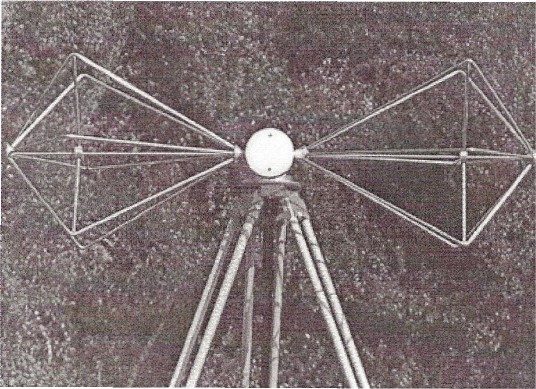
Figure 6.1. Biconic antenna for an electric field of 20 to 200 MHz
The electric signals, at the frequency of the incident fields, delivered by the sensors are injected into the measuring apparatus (spectrum analyzer and/or field intensity measuring device). The spectrum analyzer can appear essential in limit situations, for which it is a question of raising the doubt concerning the real exposure; it makes it possible for example to determine the existence of possible harmonics which contribute to the exposure and must in no way be excluded from the analysis. Moreover, their limiting values can be different from that of the fundamental frequency and, consequently, their measurement must be taken into account and not considered overall.
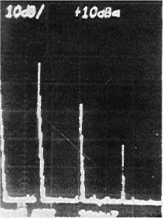
Sometimes also, it is advisable to better specify what is measured and to ensure, in particular for fields of low intensity, that the results are not generated by other remote sources of emission. This remark is true mainly for the exposure of the public, in order ensure we do not wrongly attribute responsibility to a source with suspect but “innocent” emission. Figure 6.2 provides an example of a spectrum raised near a HF press. Note that, in addition, fundamental to 27 MHz exist peaks at the harmonic frequencies of 54 MHz, 81 MHz and 108 MHz.
Figure 6.2. Frequency spectrum measured near a HF press
6.6.3. Sensors and detectors
Conditions now prevailing in the measurement field are to use specific systems, which are easy to use, require few adjustments and are light and robust. These apparatuses use special sensors better adapted to the exposure measurements than antennas and frameworks. Interested readers can to refer to the book Electromagnetic Compatibility by Pierre Degauque and Ahmed Zeddam (Degauque, 2007a and 2007b) to find all the useful information on special sensors intended for the EMC, tests of hardening to the EMI (electromagnetic impulse of nuclear origin), with lightning, electrostatic discharges and characterization of the microwaves phenomena. Below, we describe the probes or uniaxial sensors, i.e. receptors with a space component of the electric field. It goes without saying, that in order to free itself from the field polarization and to make the probe isotropic, the majority of the marketed apparatuses implement triaxial sensors sensitive to the three components of the field, in order to later allow for the calculation of the true field.
6.6.3.1. Magnetic field probes
To measure the magnetic field, we can use the Hall effect. When a current I is on, according to an axis X, in a semiconductor, subjected to a magnetic field of induction B, orthogonal according to the axis Y, a voltage VH appears in the direction Z, perpendicular to these two axes (Figure 6.3). This Hall voltage depends directly on the characteristics (resistivity and mobility) of the semiconductor, and of course on the magnetic induction field B, the electrical current I and dimensions of the probe k.
![]()
RH is called the Hall coefficient depending on the semiconductor.
Figure 6.3. Principle of a Hall effect probe: bar of semiconductor subjected to the simultaneous action of an electric field and a perpendicular magnetic induction, a field EH appears
The Hall effect probes allow the measurement of the static and alternative (until 100 kHz) fields and inductions. However, the Hall voltage varies with the ambient temperature, due to the semiconductor, which requires frequent re-calibrating. They are sensors of low dimension and high dynamics. They allow the measure to range from 100 μT to 10 T.
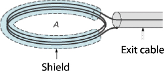
Loops and frames are systematically used in ELF, RF and UHF. The principle rests on the immersion, in a magnetic field, of a frame of varied form (round, square, trapezoidal, etc.). In the case of a coil (Figure 6.5), we recover at the exit of a loop (or n loops) of surface A, a voltage V proportional to the value of the magnetic field B of frequency v and to the developed surface of the coil (nA):
![]()
The value of V thus calculated depends on the characteristics of the coil and the frequency.
Figure 6.4. Magnetic field coil probe
The problem of the magnetic field homogenity in the zone of exposure can arise in the case of the high value field gradient (i.e. the variation of the field according to the distance). Measurement will then be affected by the dimensions of the sensor. With a loop of reduced surface, measurements will be specific corresponding precisely to the field value at the site of the sensor. With a loop of great surface, the result is in fact an average of the fields going through the loop.
Other types of sensors are sometimes used such as the magnetometers with saturable core, sensors with nuclear magnetic resonance (NMR) and magnetometers with superconductive quantum devices (SQUID). They are infrequently used for in situ measurements. They are used in research and the laboratory for very precise measurements or a determination of low intensity fields. The Faraday effect (rotation of the plan of polarization of a light wave planes crossing a material subjected to a magnetic field) is also implemented for measurement of specific magnetic fields.
6.6.3.2. Electric probes of fields
These capacitive type sensors determine an electric field by the measurement of the load or the current induced between the electrodes of an electrically insulated probe, when it is introduced into an electric field. The geometrical shapes of the electrodes are varied; the most common are rectangular or circular but they can be cubic or spherical. Subjected to a field E, sinusoidal of pulsation ω, the voltage V recovered at the boundaries of a load resistance is:
![]()
with k, constant depending on the geometrical characteristics of the probe and ε0 , the permittivity of the vacuum.
These sensors are characterized by a voltage V increasing linearly with the frequency until a high cut-off frequency, determined by the electrode's dimensions (typically 100 MHz). These sensors must be supplied by piles or batteries, i.e. a source of “floating” energy isolated electrically from the ground.
The electro-optics sensors use the Pockels effect. Crystals deprived of a centre of symmetry become birefringent under the action of an electric field. This is the case for the KDP and ADP crystals. If we have on the crystal faces, semi-transparent electrodes so that the field applied is parallel to the incident light beam, the induced birefringence is directly proportional to the electric field applied. This optical modification is converted into a signal representative of the electric field intensity by the intermediary of a system composed of a source of coherent light, an optical modulator and an optical detector. The modulated signal thus obtained is transmitted to a photodiode by the intermediary of an optical fiber and converted into an electric signal representative of the electric field.
We can use also dipoles. These are elementary antennas for which the selected length is very small compared to the minimal wavelength of the measured field. The voltage at the boundaries of the dipole is roughly equal to the product of the field in the center of the dipole by its length.
Resistive dipoles associated with thermocouples are usually used as electric field collection and detection probes.
6.6.3.3. Detectors
The signals coming from the sensors are alternative signals at the frequency of the fields. Two principal types of detectors are implemented: either by diode, or by thermocouple. The use of thermistor-bolometers is possible but is not recommended because of their thermal drift.
Detection by diode is usually performed using a Schottky diode. These diodes have a high cut-off frequency and its characteristic voltage is used either in its quadratic part for weak signals or its linear part for high signals. In the complex case, in the presence of several sources of emission or signals of high amplitude, strongly modulated, a specific correction of the indicated values is essential, the error can reach up to 5 dB. Detection by diode presents many advantages, such as a high threshold of destruction depending on the characteristics of the semiconductor, a short reaction time, the switching times can reach a picosecond and high dynamics of use (60 dB).
In the case of detection by thermocouples, we use a combination of thermocouples assembled in series. These thermocouples behave, in relation to the electric field, like dipoles, i.e. electric field sensors. A tangential electric field with the axis of a line of thermocouples induces a current involving a dissipation of heat per Joule effect creating a hot junction, a rise in temperature (with high resistance) compared to the cold junction (with low resistance) of each thermocouple. A tension is thus collected at the boundaries of each thermocouple, which added one to the other by fitting in series giving a voltage proportional to the square of the component of the electric field concerned. Generally, detection by thermocouples delivers a true effective value of the field, independent of the shape of the signal. This type of detection is well adapted to the measurement of specific fields (pulsated, modulated, etc.). However, it typically presents a relatively low sensitivity and dynamics of use of 30 dB.
6.7. Measurements
6.7.1. Measures to the static field
It is primarily the measurement of the magnetic field which must be considered; measurement of the electric field does not seem to be of interest from the point of view of health, and will thus not be described in this chapter.
Intense magnetic fields, for example, are detected in the vicinity of the tanks with industrial electrolyses. In particular, those used for the production of chlorine starting from sodium chloride, for the refining of aluminum, copper, barium, beryllium, etc. the production cells of chlorine function typically under 4.45 V with current intensities of about 90,000 A. The aluminum electrolysis tanks normally present low voltages (4.1 V) but with currents which today exceed 270 kA.
These unusual currents create static, very high magnetic fields in the vicinity of the tanks, with fast decrease of the distance d (into 1/d) but with high gradient fields. Many of these manufacturing units are currently automated; however, the presence of workers has not been completely excluded because of maintenance operations, it is thus necessary to carry out these unusual magnetic fields. A precise measurement can be taken either with saturable core magnetometers, or with superconductive quantum device (SQUID) magnetometers, or with nuclear magnetic resonance sensors. However, Hall effect sensors are, without question, better adapted and most commonly used. It is important however to direct the probe well to obtain the maximum value at a given point. We must also ensure we avoid a drift of the initial adjustment, and periodically carry out calibration using standard magnets. In addition, low dimensions of the probe allow us to localized measurements of the field and thus provide the possibility of making 3D field cartographies.
6.7.2. ELF field measurements
For measurement of the fields in the band 0 Hz to 30 kHz, the reader can refer to Bowman et al. (1998) and Laliberté (1997).
ELF fields include the frequency of the electrical network of 50 Hz (or 60 Hz) like those of the first harmonics. In fact, in this frequency band, measurements of exposure due to domestic distribution will firstly relate to the magnetic field with 50 Hz. Indeed, the magnetic field is prevalent. The electric field is of less interest, because it respects with ease its limitations.
Under high voltage lines and to a transformer, the intense currents and voltages involve the presence of strong electric and magnetic fields which it is advisable to measure. The electric fields of strong intensities, above 5 kV/m can cause indirect risks because of the human reactions associated with the discharge arcs and the currents in contact with conducting parts not connected to the ground. It is also necessary to consider the complementary risks related to the explosion and fire hazards resulting from the presence of combustible materials which can ignite under the effect of sparks or arcs generated by unprotected electric appliances. Under a powerline of 400 kV, the electric field typically reaches between 7 kV/m and 10 kV/m, above ground-level.
For the measurement of the electric field, we will use self-contained equipment (fed on battery) implementing sensors of capacitive type in the form of two half-spheres or two plates. As the measurement of the electric field is able to be influenced by the presence of the operator, the probe will thus have to be off-set using an insulating pole. The off-set sensor is connected to the measurement electronics, and thus to the display, by an optical fiber. Diplacido et al. (1978) calculated the influence of the distance from the operator compared to the sensor, under a powerline of 500 kV, and at various altitudes. It will be retained that when the operator is within less than 1 m, the disturbance is higher than 10%. It would be necessary to be held within more than 3 m for this disturbance to be acceptable.
We will use commercial apparatuses for measurements of the magnetic field, implementing field sensors (coil, Hall effect or other sensors). It is possible to use uniaxial sensors (to be directed in the field) but triaxial sensors are preferable as they are more convenient to use. We can thus take measurements of the magnetic field in front of a transformer or near an induction furnace. It will be noted that the presence of the operator has a negligible influence because human permeability is equal to vacuum permeability μ0. On the other hand, ferrous objects and great metal structures, even nonferrous, disturb the magnetic field and thus its measurement. Moreover, if the field is complex and harmonics are present, we will have to take account of it, either using an adapted apparatus, or while working with narrow band in order to measure each line of the spectrum separately.
When coil sensors are used, a coil surface of 100 cm2 will be preferred in order to conform to the normal specifications. The low-size loops can be used to measure the fields locally.
6.7.3. RF and UHF field measurements
The majority of the apparatuses implement isotropic sensors which make it possible to screen the three space components and the resulting field. The measurement of these frequencies requires us to consider two principal parameters:
– the distance between the emissive source and the zone of measurement, in order to determine if one is in the zone of Fraunhofer or that of Fresnel;
– the nature of the emissive source, namely: is it likely to have a magnetic prevalence (example of a furnace of induction or a loop of emission) or electric prevalence (example of an antenna)?
At a long distance from the source, thus in the Fraunhofer zone, i.e. beyond 1.6 times the wavelength, the reactive components of fields are almost null and only the radiated components generally remain, regardless of the nature of the emission. The plane wave conditions apply and the formulas of simplification based on the vacuum impedance Z0 = 377 ohms are operative with an acceptable precision. Below, are given some examples with plane wave conditions:
– TV broadcasting at a distance of 6 m for band I, of 1.5 m for band III and of 50 cm for bands IV and V;
– FM broadcasting at a distance of 3 m (for the frequency of 100 MHz);
– LF broadcasting at a distance of 2,000 m (for a frequency of 100 kHz);
– GSM 900 basic station at a distance of 30 cm (for the frequency of 935 MHz) and for the GSM 1,800 at a distance of 15 cm;
– for the systems using band ISM (around 2.45 GHz), like the microwave ovens, the conditions of wave planes are beyond the distance of 10 cm.
The measurement of one of the physical sizes E, H or S, involves the knowledge of both other sizes (see Table 6.7) with the following relations:

Table 6.7. Under far-field conditions, correspondence between electric field intensity E, magnetic field H and power density S
| E (V/m) | H (A/m) | S (W/m2) |
| 1 | 0.0027 | 0.0027 |
| 3.77 | 0.01 | 0.0377 |
| 10 | 0.0265 | 0.265 |
| 19.42 | 0.0515 | 1 |
| 37.70 | 0.1 | 3.77 |
| 61.40 | 0.1629 | 10 |
| 100 | 0.265 | 26.53 |
| 194.2 | 0.515 | 100 |
| 377 | 1 | 377 |
| 614 | 1.629 | 1,000 |
| 1,000 | 2.65 | 2.653 |
| 3,770 | 10 | 37.70 |
At a short distance from the source, measurements must consider all the physical quantities E, H and S, because the preceding formulas of simplification are inappropriate.
If the source is of an electric nature (for example a HF press), the electric field will be prevalent involving a high and variable wave impedance. If the source is of a magnetic nature (for example an induction furnace), the magnetic field will be preeminent and the wave impedance will be weak and unstable. In these two cases, it is imperative to separately measure the electric field and the magnetic field for a better determination of the exposure.
6.7.4. In situ measurements and total electric field
The ANFR protocol for in situ measurements, is described in detail on the website www.anfr.fr, and in a recent article by Couturier (2008). In accordance with the provisions of Recommendation ECC(02)04 (ECC, 2007), any in-situ measurement of the electromagnetic fields must be carried out at the place where the field is at a maximum. In addition, the protocol requires measurements of all the frequency bands, covering the electromagnetic spectrum with a receiver or a spectrum analyzer. Thus, we can estimate the contribution of each emission.
In the ambient environment, we saw that there are several RF radiation sources. Each source induced a certain electric field Ei (x, y, z), in a place given (x, y, z). The total field ET in (x, y, z) is:
![]()
It is this total field which it should be considered when determining if the points defined by (x, y, z) are subjected to field levels compared to the recommended limiting values, as described above in section 6.4. In Table 6.8 we provide an example drawn from measurements made in Paris by ANFR (www.anfr.fr)
Table 6.8. In a given place defined by co-ordinates (x, y, z), comparison of average effective electric field measurements, at this point, at precise frequencies with the total electric field at this point (x, y, z). The electric field total armature by the whole of the transmitters is significantly lower than the authorized limiting field here
| Frequency (MHz) | Ei (x,y,z) in V/m) | Limit values (V/m) |
| 0.8650 | 0.2443 | 87.00 |
| 94.7957 | 1.3434 | 28.00 |
| 429.0150 | 0.0378 | 28.48 |
| 567.3680 | 0.1351 | 32.75 |
| 949.6000 | 1.9208 | 42.37 |
| 2,161.6500 | 0.1235 | 61.00 |
| ET (x,y,z) = 4.0228 V/m | Limit field = 28.00 V/m |
6.7.5. Calibration
The calibration constitutes a checking of the correct operation of the measuring apparatus and, in particular, sensor (probe of field). The checking must be sufficient to detect and mitigate a dysfunction, a caused damage (the probes can be particularly sensitive to the overloads of field) or even a manufacturing defect, relating to the frequency response, the linearity and the isotropy of the apparatus. All recalibration must be done at least every 3 years (recommendation of the CEI); this time can be shorter if the manufacturer or other requirements recommend it.
Calibration is a delicate operation, and must be entrusted to accredited laboratories ISO/CEI 17 025, on the one hand, to ensure that the equipment functions correctly and was calibrated using the procedures described in metrological standards of reference, as regards exactitude in particular and, on the other hand, to ensure full documentation of the system setup quality.
Two methods are mainly used to carry out the calibration:
– The standard field method: a reference field is generated and the characteristics of this field are determined by calculation starting from the geometry of the source and the entry parameters of the generator.
– The honest standard method: in a field we initially use a standard probe, for which the traceability with the International System of Units by a standard laboratory is established, this is then replaced by the probe to be calibrated.
Calibration of the electric field probes requires the generation of well characterized fields which are obtained by means of one of the following installations:
– Capacitor plates: fitting two rectangular plates separated by a distance calculated to ensure a good homogenity of the field at the center of the equipment. This device functions correctly for frequencies up to 50 MHz.
– TEM cells (mode of transverse electromagnetic propagation): coaxial connection using a flat conductor, with a square section, which makes it possible to create an electromagnetic field easily calculable and usable until a few hundred MHz.
– Anechoïc rooms (simulation of propagation conditions of RF waves in open space): a dipole type antenna or horn generates a field in a room whose walls are covered with absorbing materials. The knowledge of the emission characteristics (power, antenna gain, positioning of the probe) allows calculation of the field. They are generally used for frequencies higher than a few hundred MHz.
The calibration of the magnetic field probes can be carried out with one of the three following equipments:
– Single coil: the intensity of the magnetic field product depends on the number of loops and the geometry of the coil flowing by an electric current.
– Helmholtz coil: it is a device used for providing a relatively uniform magnetic field, consisting of two identical circular coils on a common axis, connected in series, and separated geometrically at a distance equal to the radius of the coils.
– TEM cell: the TEM cell used for the calibration in electric field is also usable for the magnetic field.
6.7.6. Evaluation of measurement uncertainties
For all measurements of physical, chemical or biological quantity, there are no exact measurements. They can only be sullied with more or less significant errors according to the chosen protocol, the quality of the measuring instruments and operator. The results of measurements are never certain. Each result is prone to a doubt about the announced value. Uncertainty makes it possible to quantify this doubt (Priel, 1989). This is the parameter which characterizes the dispersion of the values which could reasonably be allotted to the measurand; the measurand being the physical quantity to be measured. Uncertainty quantifies dispersion, or the variation, between all the values which could be announced like result of a measurement. AFNOR (French organization official which defines the French standards which can be applied in industry or by other users) gives some tools and some methods for the evaluation of uncertainties.
Measurement of electromagnetic fields, or the powers, in the field of the non-ionizing radiations is not an exception to this general rule on uncertainties and even, by certain sides, amplifies the problems encountered because of the complexity of electromagnetism: difference between close field and far-field, variability in space (Larcheveque, 2005). In terms of the uncertainty affecting field measurements, there are four great causes, these are described in the following.
In spite of the care taken during calibration of the measurement apparatus, the calibration is affected by an absolute error. This absolute error generally appears quite negligible compared to the other sources of error, at least if the “code of practice” of the calibration are complied with scrupulously. However the generation of the reference fields used for these calibrations will never correspond exactly to the real situations met on the ground. For example, a loop used as a magnetic sensor, naturally sensitive to the magnetic field and calibrated as such, can be disturbed by the presence of an electric field, in the same way an antenna can be sensitive to the magnetic field.
The sources of uncertainty in the determination of the fields and related to the equipment used are:
– the probes do not always have a linear response according to the field, standard linearity uncertainty is estimated at 6% in relative value;
– the isotropy translates the variation with an ideal isotropic completion measurement. The case of non-isotropic antenna, uncertainty then enters within the framework of the orientation of the antenna and it is estimated at 11%; for isotropic antenna, the relative value is 9.5%;
– the factor of antenna according to the frequencies of measurement comprises, on the one hand, the calibration uncertainty and, on the other hand, uncertainty related to frequency response. The standard uncertainty is about 6% in relative value.
The environmental conditions can involve the uncertainties and in particular the uncertainties induced by variations according to the temperature and moisture. Measurements can also be affected by electromagnetic compatibility problems and, more particularly, immunity on any level of the measuring chain.
In addition when measurement is not carried out perfectly in the principal beam of the transmitting antenna the field often comes from a sum of contributions coming from multiple directions. This situation is more specifically in the cases of measurements at “indoor” or urban sites. We can then reach significant variations in the measurement of the field, when considering an uncertainty standard equal to 40% per measurement. If a statistical sampling is carried out, the law of great numbers makes it possible to divide the type-A component by √n (n being the number of measurements). Thus for 3 points of measurement, a component of relative uncertainty of 40% will have fallen to 24%, then for 100 measurements, the uncertainty of the probable type A for the measurement of the field would be 4%, type-B component not included.
The operator uncertainties can prove to be dominant if the operator intervenes without precaution and sufficient knowledge of the electromagnetism laws and equipment specifications. Due to the presence of the operator or various objects between the source and the sensor, the fields are strongly modified and movements of the operator will make them unstable. It is appropriate for the operator to moves away from the sensor to the maximum, mainly during measurement of the electric field. The palliative solutions call upon the transmission by optical fiber between sensor and electronics treatment unit, with the offset of the sensor using a pole, or better with the automation of measurements.
A bad adjustment of the apparatus or its measurement configuration could be made but will give aberrant results. The use of an unsuited measuring apparatus can give erroneous results or even involve the destruction of the apparatus. Some errors are also foreseeable if there are harmonics or frequency shifts.
Users particularly must be warned against the apparatuses using a type of sensor (for example sensitive to the magnetic field) and indicating at the same time the power density and electric field, physical quantities calculated by applying the valid formulas in plane wave. These values will be correct only in far-fields, but be completely erroneous in near-fields. In the majority of these cases, it will be necessary to separately record the values of the electric field and magnetic field with separate and suitable sensors.
All the contributions ui to uncertainty indicated earlier will make it possible to give an evaluation of the total uncertainty u. Combined uncertainty u can be evaluated according to the following formula:
where ci is the weighting coefficient (also called factor of sensitivity) generally equal to at least 1 for uncertainties related to the material.
For various reasons we express an uncertainty with a certain degree of confidence. The widened uncertainty U is then:
![]()
where k is the widening factor. The value of k is selected on the basis the degree of necessary confidence. It is 2 for an uncertainty with a degree of confidence to 95% and 3 for a confidence interval for a 99% degree of confidence (Priel, 1989).
The confidence interval in the value E of the electromagnetic field is then:
![]()
Typically, in the case of electromagnetic field measurements, standard uncertainty on the isotropy is 10%, on the linearity is 6% and on the flatness of the gain curve is 6%. The combined uncertainty u is then 13%. Using a confidence interval of 95%, i.e. k = 2, for moderate and realistic individual uncertainties, we then obtain a total uncertainty U of the field measurement estimated at 26% (Couturier, 2008).
When using a spectrum analyzer associated with a dipole (standard uncertainty ui induced by the external parameters is then dominating, 40/√n for n measurements), widened uncertainties are much stronger:
– if only one point of measurement is used, total uncertainty for a confidence interval of 95% is about 86%,
– if the operator uses three points of measurement, total uncertainty is improved but always, nevertheless, 55%.
In conclusion, in electromagnetism, the field value uncertainties can be very high. It is not uncommon for measurements to be affected by an uncertainty of more than 50% it is thus necessary to note the matched measurement results for the estimate of inherent uncertainty.
The measurement results are used to declare the conformity of the environment to the specifications. However, any experimental result sullied with an uncertainty, the decision of conformity, or not, of an environment must take into account measurement uncertainty. For questions relating to safety, it is reasonable to declare nonconformity when there is a doubt, i.e. when the results of measurements are in a zone of uncertainty. In addition, the fields (or power) in electromagnetism vary spatially (Larcheveque, 2005). It is absolutely necessary for the declaration of conformity to give the field values (or power) with widened uncertainty evaluated maximum measured in space considered to declare conformity or nonconformity.
6.7.7. SAR and its determination
In the field of intermediate and high frequencies, the basic restriction is defined by the SAR. SAR is the rate at which energy is absorbed in body tissues per unit of mass. It is expressed in watt par kilogram (W-kg−1). SAR is the dosimetry measurement widely used at frequencies above 100 kHz.
If the whole body is exposed to the far-field radiation , the average DAS is given by the relationship between the total power absorbed by the body and its mass (it is the whole body average SAR). When it is only part of the body, under conditions of close field, localized DAS is always evaluated on a mass of reference which will be either 10 g or 1 kg according to the area of the body concerned (head and torso).
SAR determination requires the use of an intrusive probe, which is difficult for human beings. In fact, we use a phantom with the shape and the dielectric properties remain close to that of a human being. The electromagnetic field would be appreciably propagated in the same manner in this phantom and a true man. Sensors suitably placed in the phantom measure the absorbed power by means of the electric field and/or the temperature (Figures 6.5 and and 6.6).
The effective SAR measurement is expensive, complicated and can be sullied with large errors (reproducibility of the fluids, of the form, position of the probe, position of the transmitter, etc.). Measurement equipment control, for the evaluations of SAR on the human body, allows a total uncertainty of about 30% (CENELEC, 2001), subject to using perfectly homogenous liquids and a perfectly definite phantom.
A measurement protocol was drawn up but it was conceived within the framework of mobile telephony and is applied with difficulty to other radio frequency applications, such as the keyboards of computers, WiFi routers, babyphones etc. Indeed, SAR measurement finds its full significance only in near-field conditions, i.e. for devices used in the immediate vicinity of the body. When the apparatus is in the far-field, the reference level to be measured is the level of the electric field.
Figure 6.5. Phantom head: against the ear is the portable terminal whose position is adjustable. The top of the cranium is bored to allow the introduction of the liquid with propagation wave properties identical to those of the human brain and also allowing the introduction of the probe (source: ABRET/Health and RF Foundation roadshow)
Figure 6.6. The probe introduced into the cranium has adjustable positions (source: Joe Wiart, Orange Labs)
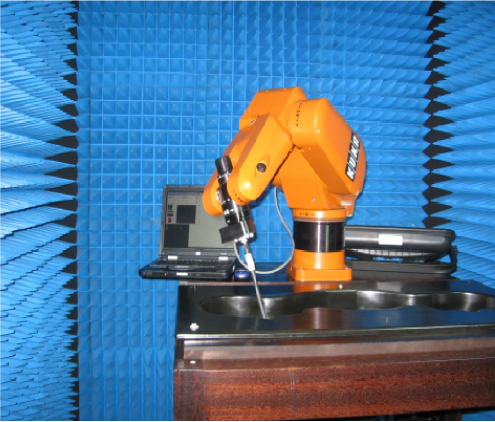
6.7.8. Measurement techniques for electromagnetic compatibility (CEM) in the field of RF
Here we describe the measurement techniques used for electromagnetic compatibility, which are also applicable to the field of dosimetry. Chapter 10 and Degauque (2007), provide detailed descriptions of these measures. In CEM, the objectives are:
– measurement of the electric and electromagnetic signals not intentionally produced by a device, and its conformity to a standard;
– characterization of the electromagnetic environment, to characterize the sources of disturbance in a given environment. The objective being to evaluate the electromagnetic constraints to which any apparatus or system placed in this medium can be subjected;
– measurement of immunity.
The CEM is a significant stage in the development of a device or electronic system and its homologation in the framework of a standard, knowing that a standard CEM describes the objective of the tests to be undertaken, the environment, the instrumentation, the characteristics of the waves, the calibration and the test procedure. The electromagnetic compatibility measurements primarily consist of giving the intensity of E and H, to the specified distances, determined with the means of broadband antennas connected to a spectrum analyzer. These measurements are then confronted with the limits imposed by the standards.
Measurements in open space are used to characterize the electromagnetic disturbances radiated by apparatuses in the frequency band of 30 MHz to 1 GHz. The reproducibility of measurements at such sites is closely related on the characteristics of the ground, ambient noise, built environment, antenna localization, etc. The measurement site of the CEM must be a priority in a quiet geographical area with the electromagnetic direction. Measurements must be done under far-field conditions for the frequencies considered (for example the distance of the antenna-apparatus must be higher 30 cm for the frequency of 1 GHz and 50 m for a frequency of 100 kHz).
To protect ourselves from the effects of the electromagnetic environment, we can use the properties of the Faraday cage: a metal cage placed around electrical equipment to protect the equipment from electromagnetic fields. An anechoic room is a Faraday cage whose internal walls are papered electromagnetic absorbents, reducing any formation of stationary waves inside the enclosure. We then approach a site in ideal open space (availability, reproducibility, disturbances outsides, climatic independence, etc.). For a detailed description of these rooms refer to Kone (2007).
A reverberating room with mode mixing (CRBM) consists of a metal enclosure (Faraday screen room) of great dimension compared to the wavelength in which a brewer of modes is installed. Contrary to the anechoic rooms, we now seek to create an electromagnetic environment of stationary waves (reflective walls). The brewer is revolving in the enclosure. In this unit, illumination is practically isotropic and the electric field is almost homogenous in average value with known margins of uncertainty (calculated). This makes it possible to generate high electric fields, although using low powers of emission (for example 100 V/m for 5 Watts). The electromagnetic test result do not depend then, except for the statistical uncertainty, on the position or the orientation of the object placed in a reverberating room.
The use of electric field or magnetic field sensors is common for the detection of very active areas, at the level of electromagnetic radiations. Localization of these zones is easy if elementary sensors are used, their displacement is simple and thus makes it possible to make a cartography of the electromagnetic local environment. Measurement in near-field is only qualitative, but it makes it possible to locate the zones potentially responsible for the possible radiation excess. This type of diagnosis is made with probes such as magnetic loops or elementary electric dipoles.
An interesting part of these measurements in close field relates to the measurement of the radiations resulting from the integrated circuits or printed circuit boards. A microprocessor, with strong transistor integration, has intense activity related to the current consumption during the phases of commutation. In the industry of the semiconductors, completely automated systems make it possible to produce the field cartography with circuits measurements (see Chapter 10).
6.7.9. Measurements for WiFi (IEEE 802.11) technologies
Radio local area networks are becoming one of the principal solutions for wireless LAN: corporate networks, hot spots, networks domestic, etc. They increase in flow, one reaching even 100 Mbits/sec. These networks, also called WLAN (wireless local area networks), based on the standard IEEE 802.11, constitute a practical connection solution, offering mobility, flexibility and low cost of deployment and use. The local area network is a system of transmission conceived to ensure a connection using the wireless links that is independent of the site of the peripherals. These local area networks develop in the university campuses and public zones such as libraries, stations, airport terminals, hotels, etc., allowing any person with a portable computer to reach services of information and to connect themselves to the Internet through the WiFi network (Labiod, 2004, Labiod 2008). In residential environments, measurements of radioelectric field and flow rates allow us to chart in 3D the fields in this environment. It is pointed out that in such environments, we are always at distances higher than the emission wavelength of the radio wave with 2.45 GHz (12.5 cm).
We give an example in the residential environment (Sizun, 2009). The emission box delivers data either with 2.4 GHz (WiFi 802.11 b/g) with a power of 100 mW, or 5.2 GHz (WiFi 802.11a) with a power of 200 MW. The measurement microcomputer is provided with a WiFi Cisco Air-cb21ag-E-k9 (802.11 ab/g) chart. Figure 6.7 gives the distribution of power observed in various places on the ground floor of a house. The emission terminal is located on the first floor, it is materialized by a star.
For specific uses when the transmitter-detector distances are lower than the wavelength (12.5 cm), determination of the fields must then call upon direct measurements of the specific absorption rate. These specific cases, characterized by a short distance between the user and the emission antenna, correspond typically if the user transfers files from his microcomputer poised on a table or his knees towards another user via a WiFi terminal (box or antenna).
Figure 6.7. Space distribution of the field power at the ground floor of a house. The WiFi terminal is located on the floor above and its position is materialized by a star. The terminal emits to 2.45 GHz, a power of 100 mW. The powers in this floor go from a few hundred μW (square −45–50) to several μW (square −60–67). Each square represents a square of 1 m sides
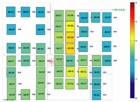
6.7.10. Field measurements in mobility situations
6.7.10.1. Measurement techniques
When the transmitter or the receiver is mobile, the measurement techniques of wave propagations makes it possible to better include/understand the various mechanisms of propagation in various environments – urban dense, rural, mountainous or different – and then to model them to envisage and optimize the communication systems and in particular those of the radio mobiles. These techniques are described in detail in Chapter 8, with a description of field measurements in narrowband, impulse response measurements, arrival angle measurements and measurements of the transmission.
6.7.10.2. Individual dosimetry – personal dosemeter
As the individuals are mobile and the fields are not homogenous in space, it is interesting to follow according to their mobility, the radiations to which they are individually subjected, also taking account of time, localization, frequencies, the field levels, etc. All of these considerations lead to the desired use of portable individual dosimeters (which are light, compact and inexpensive). ANTENNESSA (2009) thus developed a personal dosimeter, called 3RD SPY, for measurement of the electromagnetic radiation. This equipment allows us to measure in volt per meter the total electromagnetic radiation, by frequency bands, which immerge in the vicinity.
The dosimeter is a small apparatus which can be carried attached to a belt (Figure 6.8). Uninterrupted measurements are thus made, whether the carrier is mobile or not. The accumulated data are then read and memorized on a microcomputer. These portable and personal apparatuses make it possible to distinguish between the emissions from twelve transmitting sources: GSM, FM, TV, UMTS, DCS, etc. (Table 6.9). Measurements are done on a dynamic of 40 dB between 0.05 V/m and 5V/m. This dosimeter is equipped with an isotropic probe, i.e. is able to receive with the same profit an electromagnetic wave regardless of its arrival direction and polarization. German company Maschek (2009) also develops a personal dosimeter, Esm-140, with comparable performances.
Table 6.9. 12 transmitting sources accessible by 3RD SPY
| Service | Frequency band (MHz) |
| FM | 88 – 108 |
| TV3 | 174 – 223 |
| TETRA | 380 – 400 |
| TV4 and TV5 | 470 – 830 |
| GSM Tx | 880 – 915 |
| GSM X-ray | 925 – 960 |
| DCS Tx | 1,710 – 1,785 |
| DCS X-ray | 1,805 – 1,880 |
| DECT | 1,880 – 1,900 |
| UMTS Tx | 1,920 – 1,980 |
| UMTS X-ray | 2,110 – 2,170 |
| WiFi | 2,400 – 2,500 |
Figure 6.8. Individual dosemeter
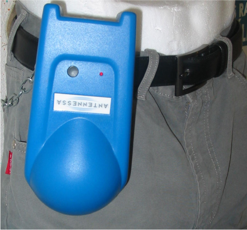
6.8. Control stations and uninterrupted electromagnetic measurements: towards a 3D electromagnetic land register
To meet the population's need for information, cities are more frequently equipped with fixed stations for electromagnetic field measurement, that measure uninterrupted and record the results on the Internet. These stations make it possible to memorize and restore the collected data. Information is collected every 24 hrs. Internet access to the data on electromagnetic quality of the environment can thus be accessible to everyone. ANTENNESSA thus equipped several cities in France and Europe. ANTENNESSA developed a single product on the market, INSITE box, which not only makes it possible to measure in-situ the level of field, but also to identify the transmitting band (FM, TV, TETRA, GSM, DCS, UMTS, WiFi, etc.). This single and patented technology makes it possible to improve the precision of the information collected while using a material which is light, less expensive and more accessible than a system with spectral analysis. The data are memorized in a completely autonomous way, and transferred completely uninterrupted; the influence of the environment on the quality of the results is then considerably reduced. ANTENNESSA thus equipped several cities in France (Brest, Marseilles, etc.) and in Europe (Valladolid, Balearic Islands, etc.).
In Greece, there are two automatic networks for the control of field radio frequencies – networks are built on a countrywide scale (Gotsis, 2008) – which made it possible to make, since November 2002, more than 4 million electric field measurements in 100 kHz – 3 GHz, 100 kHz – 900 MHz and 900 MHz – 3 GHz the frequency bands. All measurements provide fields much lower than the levels of reference and 90% of these measurements indicate fields lower than 3 V/m. The values of the measured fields do not seem to depend on localization in the country, but rather on the relative position of the source of emission and the measuring apparatus. The most significant sources of emission downtown are the FM transmitters, TV and then the basic stations of mobile telephony networks.
In Italy a electromagnetic field control network (Troisi et al., 2008) is deployed with the aim of informing public opinion and showing that the systems of RF emission are in conformity with the regulations in force in the country. All the collected data are accessible on the site www.monitoraggio.fub.it.
All of these measurements lead to an electromagnetic cartography of the country indicating in time the real electromagnetic situation and possibly showing the critical zones to correct them quickly.
This approach of electromagnetic measurements on more or less complex sites should lead in the long term to obtaining true electromagnetic cartographies in 2D or even 3D, visible cartographies uninterrupted. This lets us foresee the creation, in towns, of new services “electromagnetic registers in 3D” making it possible for the inhabitants to know at every moment via computer the cartography of the electromagnetic fields of space relating to it not only in 2D but also in 3D.
6.9. Appendix 1 – some field measurements (http://www.who.int)
– Bayphones: 8.5 V/m at 20 cm.
– Bluetooth: 0.1 V/m at a distance of 1 m from the Bluetooth peripheric.
– WiFi routers: 1.2 V/m at a distance of 1 m from the router.
– Keyboard and wireless PC mouse: 30V/m from 1 cm to the periphery.
– GSM phone: 100 V/m from 1cm to the terminal, during a communication.
– DECT: 10V/m permanently from 20 cm to the base station.
– Base-station antenna (GSM): 0.6V/m from 80 meters to the antenna.
6.10. Appendix 2 – principal characteristics of mobile communication systems
Specifications of mobile communication systems are carried out by international organizations like the ITU (www.itu.int), European Telecommunication Standards Institute (ETSI, www.etsi.org), or Institute of Electrical and Electronics Engineers Standards Association (IEEE SA, www.standards.ieee.org).
6.11. Bibliography
ANFR, ANFR/DR 15-2-1, www.anfr.fr, 2005.
ANTENNESSA, http://www.satimo.com, 2009.
Alliot J.-C., Sources de bruit, Compatibilité électromagnétique 1, Collection Technique et Scientifique des Télécommunications, Hermes – Lavoisier, pp. 31 – 184, 2007.
Balzano Q., “Exposure metrics for RF epidemiology: cellular phone handsets”, Radiation Protection Dosymetry, vol. 83, pp. 165 – 169, 1999.
Boithias L., Azoulay A.. Mesures de champ électromagnétique. Techniques de l'Ingénieur. Traité Télécoms, E 6 140, 1988.
Bowman J.D., Kelsh M.A., Kaune W.T., “Manual for measuring occupational electric and magnetic field exposures”, US Department of Health and Human Services, Cincinnati, 1998.
Cavelier C., Vautrin J.P., “Mesure des interactions ondes électromagnétiques-milieu vivant”, RGE, vol. 88, no. 9, pp. 703–709, 1979.
CENELEC EN503612, “Basic standard for the measurement of specific absorption rate related to human exposure to electromagnetic fields from mobile phones”, 2001
Challis L.J., “Mechanisms for interaction between RF fields and biological tissue”, Bioelectromagnetics supplement, vol. 7, pp. S98 – S106, 2005.
Couturier F., Mesures in-situ de champs électromagnétiques, in F. de Fornel and P.-N. Favennec (eds.), Mesures en électromagnétisme, Collection I2M, Lavoisier, pp 39–56, 2008.
Degauque P., Zeddam A., Compatibilité électromagnétique 1, des concepts aux applications, Collection Technique et Scientifique des Télécommunications, Hermes-Lavoisier, 2007a.
Degauque P., Zeddam A., Compatibilité électromagnétique 2, des concepts aux applications, Collection Technique et Scientifique des Télécommunications, Hermes-Lavoisier, 2007b.
de Seze R., Effets biologiques et sanitaires des fréquences intermédiaires, Environnement Risques et santé, pp. 31–35, 2006.
Diplacido J., Shih Ch., Ware B.J., “Analysis of the proximity effects in electric field measurements”, IEEE Trans. Power Appar. and Systems, vol. 697, pp. 2167–2177, 1978.
ECC, “Measuring non-ionizing electromagnetic radiation (9kHz-300 GhZ)”, Recommendation ECC(02)04, 2007.
Gotsis A., Papanikolaou N., Komnakos D., Yalofas A., Constantinou P., “Non-ionizing electromagnetic radiation monitoring in Greece”, Annals of Telecommunications, vol. 63, pp. 109 –123, 2008.
ICNIRP, “Guidelines for limiting exposure to time varying electric, magnetic and electromagnetic field (up to 300 GHz)”, Health Physics, vol. 74, pp. 494–522, 1998.
ICNIRP Statement, “ICNIRP statement on EMF-Emitting new technologies”, Health Physics Society, pp. 376–392, 2008.
Italian Electrical Committee, no. CEI 211–7, 2001.
Keifets L.I., van Devanter T.E., Lundell G., Swanson J., “The precautionary principle and EMF: implementation and evaluation”, Environnement Risques Santé, vol 5, p. 43, 2006
Kone L., “Techniques de mesure en compatibilité électromagnétique”, in P. Degauque and A. Zeddam (eds.), Compatibilité électromagnétique 2, Collection Technique et Scientifique des Télécommunications, Hermes-Lavoisier, pp. 107–216, 2007.
Labiod H., Afifi H., De Bluetooth à WiFi, Collection Technique et Scientifique des Télécommunications, Hermes-Lavoisier, 2004.
Labiod H., Wireless Ad Hoc and Sensor Network, ISTE – John Wiley & Sons, 2008.
Laliberte L., Guide d'utilisation d'instruments pour la mesure du champ magnétique à 60 Hz dans le milieu industriel. Rapport IRSST R-178, Montreal, 1997.
Laliberte L., Guide d'utilisation d'instruments pour la mesure des champs électriques et magnétiques émis par les machines industrielles chauffant par perte diélectrique, 1998.
Larcheveque E., Dale C., Wong M.F., Wiart J., “Analysis of electric field averaging for in situ radiofrequency exposure assessment”, IEEE Transactions on Vehicular Technology, vol. 54, no. 4, pp. 1245–1250, 2005.
Maschek, http://www.maschek.de, 2009.
Pajusco P., “Propagation channel models for mobile communication”, C. R. Physique, vol. 7, pp. 703–714, 2006.
Person C., Le Pennec F., Luc J., “Design, modelisation and optimisation of high efficiency miniature E-field probes performed on 3D ceramic prisms for SAR evaluation”, Annals of Telecommunications, vol. 63, pp. 44–53, 2008.
Priel M., Incertitudes de mesure et tolérances, Techniques de l'ingénieur, R 285, 1989.
Sizun H., Radio Wave Propagation for Telecommunication Applications, Springer, 2003.
Tanzi T., Delmer F., Ingénierie du risque, Hermes – Lavoisier, 2006.
Troisi F., Boumis M., Grazioso P., “The italian national electromagnetic field monitoring network”, Annals of Telecommunications, vol. 63, pp. 97–108, 2008.
Varsier N., Wake K., Taki M., Watanabe S., Takebayashi T., Yamaguchi N., Kikuchi Y., “SAR characterization inside intracranial tumors for case-control epidemiologic studies on cellular phones and RF exposure”, Annals of Telecommunications, vol. 63, pp. 65–78, 2008.
Vautrin J.-P., Mesurage de l'exposition humaine aux champs électromagnétiques, Techniques de l'ingénieur, 2001.
Wiart J., Dale C., Bosisio A.V., Le Cornec A., “Analysis of the influence of the power control and discontinuous transmission on RF exposure with GSM mobile phones”, IEEE transactions on Electromagnetic Compatibility, vol. 42, 531–538, 2000.
Wiart J., Watanabe S., Correira L.M, “Health protection and RF exposure assessment: engineering aspects”, Annals of Telecommunications, vol. 63, 2008.
Wong M.F., WIART J., “Modelling of electromagnetic wave interactions with the human body”, C. R. Physique, vol. 6, pp. 585–594, 2005.
1 Chapter written by Pierre-Noël FAVENNEC.
1 A window effect can be illustrated by the case of vision: humans see in one wavelength range only from 0.4 μm to 0.8 μm.
2 It should be noted that the States, members of the Union, have always faculty to envisage a level of protection higher than that envisaged by the present recommendation (Italy in use).
3 The average value is evaluated on a section of 1 cm2 perpendicular to the current direction.
4 The average SAR is measured on a time duration of 6 minutes.
5 The mass considered to evaluate the localized average SAR is 10 grams contiguous tissue.
6 For frequencies from 100 kHz to 10 GHz, the average values of the power density must be measured on a time interval of 6 minutes.
7 Figure 7.3 in Chapter 7.
8 Figure 7.4 in Chapter 7.