
Chapter 4
Low Coherence Interferometry1
4.1. Introduction
Optical wave frequencies are very high, the eye and other detectors respond to light intensity only, in other words to the time average of the electric field amplitude squared. For this reason, we almost totally miss the sinusoidal wave character of light in our daily life. In order to get full access to the phase of a lightwave experimentally, it is necessary to use interferometric techniques. Two centuries after Young and Fresnel's experiments, interferometry remains a very active domain of research: more precisely, the definition of new measurement systems. The reason for this vivid activity is the fact that the phase of a light wave is a real goldmine of information about the media through which this wave has been propagating since it is proportional firstly to the propagation distance inside the media, and secondly to their refractive index. Therefore, any change in the propagation distance of a wavelength fraction can be detected in the phase, and we can for this reason proceed to very precise measurements of small displacements. As far as the refractive index is concerned and bound to the structure of a material, any external strain (heat, pressure, electric field, etc.) modifying this structure also modifies the refractive index, and therefore the phase. If we then have a relevant theory connecting the phase with the constraint and successful inverse methods, it is possible to find the constraint applied by the phase measurement. Finally, the studied system is generally weakly perturbed by the measurement due to the nature of the interaction between light and matter.
For all these reasons, interferometric methods cover a large number of domains as diverse as biology, hydrodynamics, astronomy or still mechanics. It is advisable at this level to distinguish two types of interferometric devices: free space interferometers and fiber optics interferometers.
Even if the interference mechanisms are indeed the same in both types of devices, they each possess specificities, and thus deserve separate descriptions and very different application domains. There is plenty of literature on interferometry in free space (see, for example, Robinson et al., 1993 and the references included in the recent special edition of Optics and Lasers in Engineering, Patil et al., 2007). That is why we shall restrict our paper to the case of fiber optics devices and more particularly to low coherence light interferometry and the optical frequency domain reflectometry, which are the methods used most frequently.
Initially, only the interferogram envelope was recorded. Fiber optics interferometry was limited, therefore, to a high resolution version of the temporal reflectometry, essentially leading to the localization of defects in a component with a precision of the order of ten microns. The first phase measurement was achieved in 1989 (Francois et al., 1989), by means of a Mac-Zehnder apparatus opening the way for determination of the birefringence and chromatic dispersion of components. This approach was then adapted to devices in reflection (Dyer et al., 1999). Today, the techniques of reflectometry/interferometry are usually employed to provide spectral as well as local characterizations of fibered components.
4.2. Phase measurement
In the last ten years, two methods of phase measurement appeared in fiber optics. The first is represented by the acronym LCI, for “low coherence interferometry”; the second by OFDR, for “optical frequency domain reflectometry”. These two methods lead to results of a different nature, but have certain characteristics in common. In particular, in the different variants of one or the other method found in the literature, we find an optical system derived from the Michelson interferometer (or Mach-Zehnder) similar to the system in Figure 4.1.
The light wave transmitted by the source is divided into two waves through a −3dB coupler, and is respectively steered towards the arm containing the component under test (the test arm) and the arm containing a reflection standard (the reference arm). The waves reflected by the test and reference arms are then recombined by the coupler and interfere on the detector. The detector is controlled by a sample-and-hold acquisition circuit, often triggered by a fringe counter interferometer ensuring a regular sampling of the data. The light intensity detected by this system is given by:
[4.1] ![]()
Figure 4.1. Phase measurement system
where E(t) is the electric field of the incidental wave, τ is the delay between the reflected waves and rr and rt is the reflection coefficients, in amplitude, of the reference arm and the test arm respectively. The first two terms of this relation are of no interest because they refer to intensities from which any notion of phase has disappeared. On the other hand, the last term being directly proportional to the reflection coefficient provides information on the amplitude and the phase of this coefficient. The objective of the data analysis is then to invert relation [4.1] and extract these two parameters.
4.2.1. Low coherence interferometry
The light sources used in LCI optical systems are low coherence sources (superluminescent diodes or amplified spontaneous emission sources), whose spectral width is typically around thirty nanometers. Given the weak coherence of the source, the interferences occur within a small distance, of the order of about twenty micrometers, around the position of equal optical path in the test arm and the reference arm. It implies that to probe a component's entire length, it is necessary to change the optical road in the reference arm.
It is possible to build a device with only fibers: for example, by rolling the fiber of the reference arm around a piezoelectric bar in order to stretch it, applying a voltage across the bar, but it remains delicate, notably because the chromatic dispersion of the fiber causes a different optical path variation for the various wavelengths. So the reference arm is generally in free space. The variation of the optical path is then made by means of a mobile mirror moving along an axis. However, for certain applications in ophthalmology requiring very fast acquisitions, a delay line with the delay based on a rotating prism has been designed to reach a speed of 176 m/s (Delachenal et al., 1997; Szydlo et al., 1998; Delachenal et al., 1999).
The data analysis requires a stable and regular sampling of interferograms. Most of the time analysis is undertaken by means of an auxiliary interferometer using a laser stabilized in frequency and serving as a fringe counter. It is then possible to track down the exact movement of the mobile mirror, and to regularly sample the signal of the fiber interferometer. However, as the interfringe depends on the refractive index of ambient air, it is necessary to determine this last refractive index exactly. This can be done measuring the temperature, the pressure and the humidity ratio and the Eldén relations (Elden, 1966).
The electric fields Et and Er, of the waves reflected from the test and reference arms respectively, are given by:
[4.2] ![]()
where σ is the wave number, Lr,t(σ) the optical paths of the reference and test arms and ρ(σ) the amplitude spectral density of the electric field. All the functions depending on the wave number have been analytically expanded in the negative frequencies so that f(−σ) = f*(σ). Since the detector acts as an integrator over a long time, compared to the coherence time of the light source, the intensity is the average time of the total instantaneous intensity:
![]()
The variable part of the intensity is then given by:
[4.3] ![]()
where x stands for the reference mirror displacement and ![]() for the Fourier transform. S(σ) = rr(σ)|ρ(σ)|2 is the radiant power spectral density of the source filtered by the system, and φ(σ) corresponds to the phase shift bound to the optical path difference between the two arms. This relation is the basis of the measurement analysis. It shows that the terms rt(σ) and φ(σ) can be determined from the Fourier transform of the interferogram.
for the Fourier transform. S(σ) = rr(σ)|ρ(σ)|2 is the radiant power spectral density of the source filtered by the system, and φ(σ) corresponds to the phase shift bound to the optical path difference between the two arms. This relation is the basis of the measurement analysis. It shows that the terms rt(σ) and φ(σ) can be determined from the Fourier transform of the interferogram.
The term φ(σ) contains the entire phase accumulated by the wave during its return in the reflectometer and the sample under test. To determine the phase shift due only to the sample, it is necessary to undertake an initial measurement without the sample, which gives the phase shift caused by the interferometer. We then connect the sample and proceed to a second measurement. The phase shift φe(σ) = 2π ne(σ) ![]() e σ created by the sample can be obtained simply by subtraction.
e σ created by the sample can be obtained simply by subtraction.
The group delay, which corresponds to the time it takes for the wave packet to propagate through the sample, is defined by τg = (le/2πc) d k/d σ, where k is the module of the wave vector: k = 2πne(σ) σ. The group delay is thus directly connected with the first derivative of the phase, to which constant and generally indefinite terms are added. In practice, only variations of the group delay are important. Adding constant terms to the group delay consists of adding a given propagation length in vacuum, which does not cause dispersion. This is the reason why only the relative group delay will be considered in the following. Relative group delay is simply given by:
[4.4] ![]()
The dispersion being defined as Dσ = − (σ2/![]() e) d τg/d σ, it can also be derived from the interferogram phase measurement:
e) d τg/d σ, it can also be derived from the interferogram phase measurement:
[4.5] ![]()
4.2.2. Optical frequency domain reflectometry (OFDR)
The light source used in OFDR is a tunable laser whose optical frequency is a linear function of time. As the light at a given moment is very coherent it does not impose limitations concerning the path difference, so the reflector of the reference arm is fixed. Some systems (Choma et al., 2005) do not need a second arm in the interferometer as a reference reflector is inserted into the test arm, which maximizes the path common to both interfering waves, and thus, reduces the phase noise. The intensity which is recorded can be written as follows (Yun et al., 2003):
[4.6] ![]()
where z is the coordinate along the longitudinal axis of the sample under test, and σ(t) is the instantaneous wave number. Г(z) is the coherence function of the laser instantaneous output signal. Г(z) ideally = 1, but in practice its amplitude decreases with z, which limits the depth of measurement. Finally, r(z) and φ(z) are the amplitude and the phase of the sample local reflection coefficient, respectively.
Since the wave number varies linearly with time: σ(t) = σ0 + αt, we have a situation similar to LCI, where the intensity is expressed as the Fourier of the complex reflection coefficient of the component under test. We can thus use comparable methods to determine the reflection coefficient and derive the group delay and the chromatic dispersion of the sample.
The OFDR methods were initially considered as intermediate methods between the LCI and time of flight techniques. Today, with the improvement of laser sources concerning their line widths and the linearity of frequency variation, the OFDR system resolution is comparable to the LCI resolution. OFDR systems then tend to supplant LCI systems because they present some advantages, like a greater ease of operation (no need for mechanical displacement elements) and a higher sensitivity (Leitgeb et al., 2003).
4.3. Metrology considerations
4.3.1. Wavelength
As was previously shown, phase measurement by interferometry allows analysis in the Fourier space and thus for studies in spectroscopy. The precision of the wavelength measurement is then a determining parameter. In this section we shall present the results of two studies on this subject.
The first study was initiated by the National Institute of Standards and Technologies (“NIST Telecom Round Robin”). Ten laboratories from different countries around the world were involved (Rose et al., 2000) The purpose of this action was to compare the fiber Bragg gratings characterization methods. The participants used essentially common optical spectrum analyzers to measure the reflection spectrum of two standard gratings and a “phase shift” device (Costa et al., 1982; Genty et al., 2002) to measure their group delay. This technique consists of modulating the incident light wave and measuring the phase shift of the wave which propagated through the sample under test. These gratings have also been characterized by LCI at NIST and later in our laboratory.
The central wavelengths and the −3 dB bandwidths of the two gratings have been tested, and the results obtained from the participants in the NIST Telecom Round Robin and those obtained in our laboratory (noted LCI in the table) are recorded in Table 4.1. We observe an excellent agreement between the LCI measurements and those obtained by classical methods. The wavelength difference does not exceed 10 pm.
The second study was carried out on a mux/demux commercially available from NetTest using a diffraction grating in a free space configuration. The tested multiplexer makes a multiplexing of one channel input towards 16 channels output. This component is athermalized and calibrated according to the ITU standards. It can therefore be used as standard. According to the manufacturer, the channel
Table 4.1. Center wavelength and bandwidth of reference fiber Bragg gratings
| ITU Grating | Chirped Grating | |
| λLCI (nm) | 1, 552.51 ± 0.01 | 1, 551.56 ± 0.01 |
| λRound Robin (nm) | 1, 552.521 ± 0.008 | 1, 551.57 ± 0.06 |
| ΔνLCI (GHz) | 52.85 ± 0.01 | 2,017 ± 11 |
| ΔνRound Robin (GHz) | 51 ± 3 | 2,018 ± 7 |
spacing is 100 GHz and the — 1 dB bandwidth of each channel is at least 28 GHz. The measurement of the multiplexer response is made channel per channel. The tested channel is connected to the test arm of the reflectometer. The light coming from the reflectometer is coupled into the multiplexer where it is reflected by the grating and coupled in the input channel which terminates in a mirror. The light wave which is reflected on the mirror propagates back toward the reflectometer along the same forward propagation path. In this configuration, the intensity which is recorded is proportional to the square of the tested channel transmission factor.
Figure 4.2. Transmission of the first height channels of a multiplexer/demultiplexer
In Figure 4.2 we show the normalized transmission factor of the first eight channels. The different channels transmissions are all Gaussian shaped with —1 dB width close to 29 GHz, or 230 pm. The peaks are regularly 100 GHz apart. These results are in perfect agreement with the manufacturer's data. The measurements of the different channels' central wavelengths is made by NetTest using a highly stable tunable source. In Table 4.2, we registered the differences between the central wavelengths measured by LCI and those given by the manufacturer. They are lower than 13 pm, we will use this value as the estimation of the exactness of the measurements.
Table 4.2. Differences between the central wavelengths of the channels
4.3.2. Relative group delay
The two standard gratings of the Round Robin may also be used as references in the group delay measurements. The curves corresponding to 10 successive LCI measurements of the relative group delay for the ITU grating and the chirped grating are represented in Figures 4.3a and 4.3b. The ITU grating relative group delay is asymmetrical and nearly flat around the Bragg wavelength. It increases on the edges, its variations of the order of 60 ps in the −20 dB bandpass. The relative group delay of the chirped grating oscillates, the amplitude and the frequency vary with the wavelength. Its peak-to-peak variation in the −20 dB bandpass is 120 ps.
Figure 4.3. Relative group delay of the reference fiber Bragg gratings inside the −20 dB bandwidth
The group delays of the ITU and the chirped gratings measured using LCI are in perfect agreement with the results obtained by the “phase shift” in their shape as well as in the amplitude of their variations. So far, the slope of the straight line Δ around which the chirped grating group delay oscillates is 6.84 ± 0.01 ps/nm with the LCI to be compared to 6.81 ± 0.04 ps/nm with the “phase shift”. The residual group delay of a chirped grating is the difference between the group delay measurement result and Δ. The residual group delay of the grating we are considering varies from 8 ps to −4 ps in the wavelength interval [1, 544 nm; 1, 560 nm] and its values obtained by the two methods decrease from about 4 ps down to 0 ps in this wavelength interval.
Figure 4.4. Group delay measurement accuracy for ITU grating and chirped grating
In order to estimate the repeatability of the group delay measurement, the difference between the average and each measurement result for all wavelengths has been calculated for a series of 10 successive measurements. We presented the distributions of the differences obtained for the ITU and the chirped gratings in Figures 4.4a and 4.4b. It can be seen that these distributions follow a normal law and the accuracy of the measurements is better than 0.5 ps, which is very small compared to the group delay variations in this wavelength interval.
4.3.3. Chromatic dispersion
The chromatic dispersion curves obtained for three optical fibers around 1.3 μm and 1.5 μm are represented in Figure 4.5. Two fibers are G652 and G655 standard fibers. The other fiber is a dispersion compensating fiber manufactured by Sumitomo. These three samples are approximately 50 cm long.
From our results on chromatic dispersion, the G652 fiber corresponds to the ITU standard. As a matter of fact, its dispersion is less than 3.5 ps/nm/km for |λ – 1.31| < 0.025 μm and less than 19 ps/nm/km at 1.55 μm. This 50 cm long G652 fiber sample is part of a 6 km fiber whose dispersion had been measured by the Bureau National de Métrologie using time domain reflectometry. The value obtained using the time domain technique is 17.3 ps/nm/km at 1.55 μm and we obtained 17.0 ps/nm/km using the LCI at the same wavelength. The G655 fiber dispersion is increasing slightly in the two wavelength intervals under consideration. It is of the order of −16 ps/nm/km around 1.3 μm and 4 ps/nm/km around 1.55 μm. The SUMITOMO fiber is designed for dispersion compensation in a 1.55 μm network: short lengths of this particular fiber may be inserted and used to compensate the other fibers' dispersion. Thus its dispersion is negative, decreasing and very high, close to −130 ps/nm/km.
Figure 4.5. Chromatic dispersion of the three optical fibers at 1.3 μm and 1.55 μm wavelengths
The measurement repeatability has been confirmed by proceeding to a large number of measurements (a hundred) on the same sample. Several short length samples of the three fibers mentioned above have been tested this way. The distributions of the differences to the chromatic dispersion average value are plotted in Figure 4.6 for the G652 and Sumitomo fibers at 1.5 μm. These curves show that the repeatability of the dispersion measurements using LCI is of the order of ±0.2 ps/nm/km. We obtained similar results on the other fibers and at other wavelengths.
Figure 4.6. Chromatic dispersion: distribution of the difference with average
4.4. Applications
4.4.1. Characterization of photonic crystal fibers
Photonic crystal fibers (PCFs) have very specific properties which are impossible to obtain with conventional fibers. The first samples were created in the 1990s and since then they have raised increasing interest. The internal total reflection PCFs are single mode broadband waveguides. With these fibers, it is possible to adjust the chromatic dispersion as well as the effective area of the guided modes and therefore the non-linear effects.
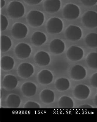
Figure 4.7. Section of a PCF: hexagonal pattern of holes with diameter d = 1.12 μm and pitch Λ = 1.42 μm
Most of these fibers have a slight anisotropy which can confer a noticeable birefringence to them. This birefringence may also, similar to other characteristics, be derived from phase measurement. In fact, when a fiber has two polarization eigen axis with different refractive indices, the light wave components polarized along these directions propagate with different velocities. The interferograms corresponding to these two polarizations are then distanced by d = 2Δn ![]() ech, where Δn is the birefringence and
ech, where Δn is the birefringence and ![]() ech is the length of the sample. The detected intensity can be written: I(x) = I0(x) + I0(x ‒ 2Δn
ech is the length of the sample. The detected intensity can be written: I(x) = I0(x) + I0(x ‒ 2Δn![]() ech), which leads to: I (σ) = I0(σ)[1 + cos(4πΔn
ech), which leads to: I (σ) = I0(σ)[1 + cos(4πΔn![]() echσ)]. Beats raise inside the spectrum whose period Δσ depends on the length and the birefringence of the sample. We may determine the group birefringence from the beat period measurement (Folkenberg et al., 2004; Ritari et al., 2004) as given by:
echσ)]. Beats raise inside the spectrum whose period Δσ depends on the length and the birefringence of the sample. We may determine the group birefringence from the beat period measurement (Folkenberg et al., 2004; Ritari et al., 2004) as given by:
[4.7] ![]()
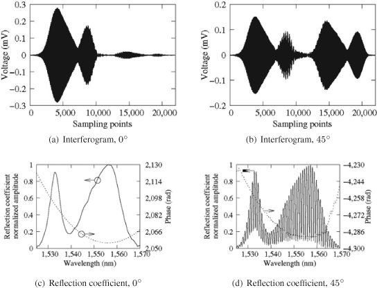
Due to this birefringence, we have to insert a polarizer in front of the detector and proceed to a preliminary measurement to identify the eigen axis of the fiber. In practice, the directions of the fiber neutral lines are given by the two positions of the polarizer which reduce the beats in the reflection coefficient modulus to zero. These positions will later be noted 0° and 90°. The chromatic dispersion along the fiber's eigen axis is measured inserting the polarizer into position 0° and 90°. In order to measure the birefringence, the polarizer position is 45° since the beat visibility is then at its maximum.
In Figures 4.8(a and b) we showed the interferograms obtained on a PERFOS PCF whose structure is a hexagonal arrangement of holes, for specified polarizer angles of 0° and 45°. A SEM picture of a cross section of the fiber is shown in Figure 4.7. The interferograms corresponding to the two eigen states of polarization can be seen when the polarizer is oriented at 45° and only one of them remains when the polarizer is 0° oriented. This corresponds to the presence of beats in the modulus of the reflection coefficient for the 45° orientation (Figure 4.8d). The beat period measurement for this fiber leads to a relatively high birefringence of (1.45 ± 0.02) × 10−3 at 1, 550 nm. By way of comparison, the birefringence of a PANDA polarization maintaining fiber is 4.2 × 10⁻⁴, the group birefringence of a PCF with 1.89 μm diameter holes 2.13 μm apart is 8.1 × 10⁻⁴ (Palavicini et al., 2005).
The sources of uncertainty are the error in the fiber length measurement and the error in the beat period measurement. This latter is the predominant error in our case. As a matter of fact, the error on the 30 cm sample length is of the order of 1 mm which causes 10−6 uncertainty on the birefringence. The error on the wavelength is a tenth of 10−12 m (Leduc et al., 2003) which corresponds to a 4 × 10⁻⁶ μm−1 error on the wave number σ. Considering that we count about fifty periods in our measurement procedure, this approximately causes a 10−5 uncertainty on the birefringence.
The measurement resolution is limited by the light source spectral width. To be able to measure the birefringence, we must observe at least two oscillations in the spectrum. The beat period must then be equal to at least 20 nm. The longest sample length we can analyze is typically of the order of 1 meter and the lowest birefringence we can measure is 6 × 10⁻⁵ with this device.
Figure 4.8. Influence of the polarizer
The chromatic dispersion of the fiber is −17.5 ps/nm/km and −15.8 ps/nm/km respectively for 0° and 90° and its dispersion slope is low and negative: −0.046 ± 0.003 ps/nm2/km along one polarization direction and −0.042 ± 0.002 ps/nm2/km along the other direction.
4.4.2. Amplifying fiber characterization
During his work on Erbium doped amplifying fibers, Desurvire (Desurvire, 1994) took an interest in the case of a fiber “pumped” by 980 nm or 1, 480 nm wavelength light waves. He predicts the variations in a propagation medium dispersion of the order of ±30 ps/nm/km for an Er3+ ion concentration of 1019 ions/cm3. These indices and dispersion variations had been observed experimentally on Lithium Niobate waveguides (Takada et al., 1992) and optical fibers (Thirstrup et al., 1996; Lupi et al., 2001). The behavior of Erbium doped fibers is very different from passive fibers behavior, due to the strong interaction between the light wave and the ions, which requires a precise model. We will follow the method proposed by Desurvire to study the interaction between light and Erbium doped fibers.
In the wavelength spectral band of the fiber (1, 530 nm − 1, 560 nm), the interaction between the light wave and the Erbium ion takes place at energy levels 4I13/2 and 4I15/2. These two levels respectively contain g1 and g2 sub-levels, whose degeneracy is raised by the ligand field induced by the vitreous matrix. The sub-levels energies are Ej, j ∈ [1,g1] and Ek, k ∈ [1, g2] eigenvalues of the internal Hamiltonian ![]() (in the following, the indices j refer to the first level and the indices k to the second level). The interaction between the light wave and the ions is described by the Hamiltonian
(in the following, the indices j refer to the first level and the indices k to the second level). The interaction between the light wave and the ions is described by the Hamiltonian ![]() , where μ is the electric dipole momentum operator and E the incident wave electric field. Two sub-levels can be coupled together in this interaction. However, due to the thermal agitation there is a constant redistribution of the populations of the sub-levels inside the same level. For this reason, the distribution of sub-level populations follows Boltzmann's law, the probability bn for the energy level En to be occupied being given by
, where μ is the electric dipole momentum operator and E the incident wave electric field. Two sub-levels can be coupled together in this interaction. However, due to the thermal agitation there is a constant redistribution of the populations of the sub-levels inside the same level. For this reason, the distribution of sub-level populations follows Boltzmann's law, the probability bn for the energy level En to be occupied being given by ![]() .
.
The system evolution is entirely inside the density operator ρ evolution. The variations of the dielectric susceptibility ![]() induced by the interaction can then be bound to the elements of the density matrix via the macroscopic polarization:
induced by the interaction can then be bound to the elements of the density matrix via the macroscopic polarization: ![]() . Thus in steady state
. Thus in steady state ![]() . The problem is summed up by the calculation of the coherence ρjk steady state values between the levels, and of the total populations of the first and second levels
. The problem is summed up by the calculation of the coherence ρjk steady state values between the levels, and of the total populations of the first and second levels ![]() and
and ![]() . This calculation is based on the density operator evolution equation:
. This calculation is based on the density operator evolution equation: ![]() , where
, where ![]() and where a relaxation term has been added to take into account the spontaneous emission and non-radiative transitions.
and where a relaxation term has been added to take into account the spontaneous emission and non-radiative transitions.
In steady state conditions, the dielectric susceptibility variations are the result of the superposition of the contributions caused by the different possible transitions from an energy level Ek to a level Ej. Each transition is associated with a Lorentzian line ![]() whose width is Δωkj, whose pulsation is ωkj and oscillator strength is fkj, so that the total response is equal to:
whose width is Δωkj, whose pulsation is ωkj and oscillator strength is fkj, so that the total response is equal to:
[4.8] ![]()
N is the Erbium ion concentration, q and m are respectively the charge and mass of the electron. Since the interaction takes place on the total length L of the fiber, the refractive index variations related to this interaction are given by: ![]() , where η is the overlapping factor of the guided wave, n0 the host matrix refractive index and χ′ the real part of the susceptibility. The dispersion induced by the ions-light interaction is finally given by Dλ = −(λ/c) (∂2δn) /(∂λ2), and according to [4.8]:
, where η is the overlapping factor of the guided wave, n0 the host matrix refractive index and χ′ the real part of the susceptibility. The dispersion induced by the ions-light interaction is finally given by Dλ = −(λ/c) (∂2δn) /(∂λ2), and according to [4.8]:
[4.9] ![]()
where ![]() and
and ![]() .
.
Figure 4.9. Chromatic dispersion of a 50 cm long sample of Erbium doped fiber
Therefore in order to analyze the dispersion of an amplifying fiber, it is necessary to adjust the energy levels as well as the transitions widths and their oscillator strength. It is moreover necessary to eliminate the classic fiber dispersion bound to its geometry and to the variations of the matrix refractive index with the wavelength. This can be done by adjusting the phase of the reflection coefficient of the fiber using a polynomial giving the classic dispersion, which we delete from the phase we measure to retain the dispersion bound to the resonating interactions. An example of chromatic dispersion of an amplifying fiber is given in Figure 4.9 (dashed line curve). The plain line curve represents the adjustment following relation [4.9]. This adjustment required 8 energy levels whose values expressed in cm−1 are: {0; 65; 125; 192; 258; 6545; 6620; 6685; 6745}. The Erbium ion concentration given by the adjustment is of the order of 1 × 10¹⁹ions.cm−3, or 200 ppm, which is in perfect agreement with the manufacturer's data.
The LCI can be used to study the homogenity of a fiber. In Figure 4.10, for example, we show the chromatic dispersion curves of several 50 cm samples, cut and removed every 5 m along the same amplifying fiber. Almost all of the samples present the same dispersion and can be adjusted using the same procedure described above, except two of them (plain and dashed line curves). The dashed line curve is actually only different from the others by a proportionality factor of 1.8. Therefore the corresponding sample presents the same energy levels as the others but the Erbium ion concentration is nearly twice as high. On the other hand, in order to adjust the plain line curve, it has been necessary to proceed with levels of different energy:
Figure 4.10. Chromatic dispersion of several samples removed from the same amplifying fiber
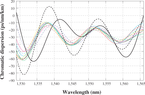
{0; 65; 110; 174; 265; 6532; 6590; 6648; 6740} (cm−1). This lets us suppose that the Erbium ion environment was locally different, causing a slightly different Stark effect degeneracy increase of the energy levels.
4.4.3. Local characterization of fiber Bragg gratings
4.4.3.1. The fiber Bragg gratings
We obtain a fiber Bragg grating shining a UV laser on a fiber that has been firstly exposed to high pressure hydrogen to increase its photosensitivity (Hill et al., 1978). Interference fringes are produced and coupled into the fiber core to inscribe a longitudinal modulation of the refractive index matched with the light intensity modulation:
[4.10] ![]()
where neff is the effective index of the propagating mode, Δnac the index modulation amplitude, Δndc the effective index average and Λ(z) the modulation pitch. One consequence is that the Bragg gratings reflect part of the incident light intensity spectrally centered on the Bragg wavelength. This latter depends on the index of the propagating mode and λ the pitch of the refractive index modulation inscribed along the fiber core:
[4.11] ![]()
Thanks to the great flexibility of photo-inscription techniques we can produce gratings with very different reflectivity leading to a large variety of applications for this component (Hill et al., 1997). For example, it is possible to inscribe gratings whose reflection spectrum is very narrow, typically hundreds of picometers. We obtain an optical multiplexer assembling in series several gratings of this kind (Jackson et al., 1993). An entirely fibered laser cavity can be achieved connecting such gratings to both ends of an amplifying fiber (Guy et al., 1995). It is also possible to inscribe gratings whose modulation pitch varies longitudinally. These gratings are said to be “chirped”. Schematically, the Bragg wavelength changes with the position along such a grating, therefore the different spectral components of the incident light reflect at different points of the grating. This property can be used to compensate the chromatic dispersion (Eggleton et al., 2000) or compress the light pulses (Broderick et al., 1997). The Bragg gratings are increasingly used as sensors (Ferdinand, 1992) because any external strain (temperature, pressure, etc.) causes a shift of the reflected light spectrum. We can determine the strain intensity from the measurement of this shift. Spectrally sharp gratings are sensors with very high sensitivities.
As this has been shown previously, we may use LCI to characterize the spectral properties of Bragg gratings. Nevertheless, this characterization is not always sufficient. The spectrum indeed gives global information on the grating, averaged over its entire length (typically some millimeters). However, we sometimes wish to have more localized information which is, as for instance in the detection of a defect in the photo-inscription or in the measurement of non-uniform constraints. The solution to this problem has been provided by the works devoted to the design of Bragg gratings, editing of many algorithms for index longitudinal profile reconstruction whose starting point is the impulse response or the complex reflection coefficient of the grating. As this last quantity was naturally obtained by LCI, it was logical to attempt to associate them both and proceed to the experimental synthesis of real gratings. This approach turned out to be fruitful and stands among the most important applications of the phase measurement in fibered optics.
Local characterization of a Bragg grating amounts to determining its average effective index Δndc(z), its modulation amplitude Δnac(z) and the variation of its modulation pitch Λ(z) — Λ0. The reconstruction algorithms which have been set up to carry out this task are generally based on the coupled modes theory (Kashyap, 1999; Sipe et al., 1994). The fiber is supposed to be “single mode” and lossless, therefore allowing the propagation of both forward and backward waves uf and ub. The action of the grating on these waves is given by:
[4.12] ![]()
where Ω(z) is the coupling coefficient of the grating:
[4.13] ![]()
with
[4.14] ![]()
where η is the mode confinement factor. In practice, Ω(z) is the coupling coefficient which is calculated using the reconstruction algorithms. We can easily deduct the modulation amplitude from this calculation as it is proportional to the modulus of the coupling coefficient. It is more difficult to determine the grating average effective index and the pitch variations. These two parameters intervene in the argument of the grating coupling coefficient Ψ(z), as they both modify the optical path seen by the wave. This implies that it is necessary to have a priori information to be able to differentiate them. If the grating is uniform, the average effective index only intervenes so that:
[4.15] ![]()
If the grating is chirped linearly (Λ(z) = Λ0 + αz) with a constant average effective index, then:
[4.16] ![]()
It is necessary to determine in a first step the chirp of the grating using a parabolic adjustment of the phase of the coupling coefficient, to be able to calculate the average effective index in a second step.
Among the numerous algorithms which have been set up to reconstruct the index profile of Bragg gratings, two are now necessary. The most frequently used algorithm is “layer peeling” (Robinson, 1975; Feced et al., 1999; Poladian, 2000; Skaar et al., 2001), which is fast and efficient. The second reconstruction algorithm occasionally used (method noted “GLM”) is based on an integral formulation of the coupling equations and on an iterative resolution of these equations (Song et al., 1985; Peral et al., 1996; Keren et al., 2003).
4.4.3.2. Accuracy of the index profile reconstruction
Combining the reflectometry measurements and the algorithms described above, it was possible to reconstruct the index profile of several real gratings of very different natures. We then proceeded to synthesize uniform gratings (Chapeleau et al., 2003) and chirped gratings (Leduc et al., 2007) and less classical gratings as well like staircase steps gratings (Chapeleau et al., 2006), crenel gratings (Giaccari et al., 2003) or gratings with phase step (Poladian et al., 2003; Chapeleau et al., 2004).
This measurement technique benefits from LCI sensitivity. It is then possible to characterize gratings with very low amplitude modulation. This is represented
Figure 4.11. Staircase step grating
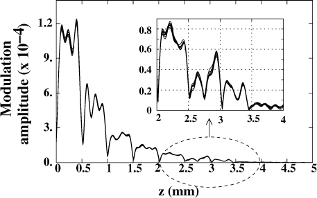
in Figure 4.11, where we show the reconstructed profile of a grating made up of 7 staircase step gratings, each step receives half the energy of the previous step during the photo-inscription.
All the steps are present in the reconstructed profile, even the last step whose amplitude is 2 × 10⁻⁵. In terms of reflectivity, the lowest limit in the reconstruction is about 1%. The highest limit is approximately 95%. This value may somehow be passed over after proceeding to several measurements. It has that way been shown that it was possible to reach 99% reflectivity by either measuring the complex reflection coefficients of the grating for both forward and backward propagating light waves and combining the reconstructed profiles (Rosenthal et al., 2003), or simultaneously measuring the complex reflection coefficient of a grating and its transmission coefficient to correct the spectrum (Rosenthal et al., 2005). The validity of the modulation amplitude measurements using this method has been proved comparing the profiles obtained by the transverse diffraction technique (Krug et al., 1995). The agreement between the two methods is always very good, within the limits in reflectivity given above. The repeatability of the measurements is shown in Figure 4.12.
These results have been obtained measuring several gratings several dozen of times. The repeatability has been estimated by calculating the max difference between the successive profiles along the whole grating: ![]() from which we derived a global estimation: emax = maxz[emax(z)] as illustrated by Figure 4.12a. The repeatability depends weakly on the reflectivity, it is around
from which we derived a global estimation: emax = maxz[emax(z)] as illustrated by Figure 4.12a. The repeatability depends weakly on the reflectivity, it is around
Figure 4.12. Repeatability of the synthesis of amplitude modulation
3% in the case of highly reflecting gratings (Rmax > 50%) and around 4% in the case of weakly reflecting gratings (see Figure 4.12b). It is difficult to estimate the propagation of noise in the inverse methods, nevertheless we may give a limit lower than the precision of the measurement. The major source of uncertainty indeed lies in the relative uncertainty of the values of Rmax and η, which is of the order of several %. We find a repeatability of the same order of magnitude.
Figure 4.13. Phase of a chirped grating measured by par LCI and GLM
In Figure 4.13, we present the phase of a chirped grating photo-inscribed through a phase mask with a 0.05 nm/cm linear pitch. We then expect that the grating is also chirped linearly with a slope of 0.025 nm/cm. In accordance with the equation [4.16] prediction, the phase of this grating is parabolic. The adjustment leads to a chirp of 0.030 ± 0.002 nm/cm. Other measurements have been done on 3 gratings photo-inscribed through another phase mask linearly chirped with a 3 nm/cm slope. In this case, we obtain the following values for the chirp: 1.428 ± 0.002 nm/cm, 1.427 ± 0.003 nm/cm and 1.428 ± 0.002 nm/cm, which are indeed all equal but slightly different from the expected value (1.5 nm/cm). At present, it is not possible to conclude whether this difference is a measurement error or an inscription defect. A misalignment or an inscription beam non-uniformity may indeed lead to the inscription of a chirp slightly different from the theoretical chirp. This study shows that when we combine reflectometry and a reconstruction algorithm we may get to the chirp of a Bragg grating, with at worst an error of several percent, which is not possible using classic methods.
When the chirp of a grating has been determined, we can calculate its average effective index using equation [4.16]. The relative reproducibility is once again several percent. The accuracy is more difficult to establish since there is no direct method of reference to measure the average effective index or theoretical values. However, the validity of the measurements can be checked indirectly. The values of the modulation amplitude, chirp and average effective index determined for a real grating may be used to simulate a theoretical grating using relation [4.10]. The reflection coefficient, in amplitude of this grating, can then be calculated using the transfer matrix method (Skaar, 2000) and compared to the reflection coefficient, which has been measured directly. In following this procedure, we obtain for all cases an excellent agreement between the two coefficients, as is illustrated in Figure 4.14. This proves the accuracy of the average effective index measurements.
Figure 4.14. Comparison of the reflection coefficients calculated from the reconstructed profile with those directly measured. The group delay curves have been translated to obtain a better readability
4.4.4. Strain and temperature sensors
4.4.4.1. Background
Since the 1990s, many research activities (Kersey, 1996; Kersey et al., 1997; Rao, 1997) have been oriented to the set up and the development of new optical sensor systems, in particular those based on Bragg gratings. These components are excellent transducers: they are very sensitive to temperature variations, pressure and strain. Moreover, their small sizes confer on them low intrusion capability inside materials and remote and distributed measurements along one fiber. They can also be used under severe environmental conditions owing to their lack of sensitivity to electromagnetic perturbations and their high resistance to ionizing radiation, corrosion and fatigue. Thanks to these many advantages, sensor systems based on Bragg gratings can be found today in many applications (Rao, 1999): such as measurements, detection, surveillance in civil engineering, aeronautics, ship building, oil industry, etc.
A Bragg grating reflects a very thin spectral band, centered on the Bragg wavelength λB given by [4.11]. The parameters neff and Λ depend linearly on the temperature and the strain applied along the grating. In order to measure a uniform variation of the temperature ΔT and the longitudinal strain ∈ using a Bragg grating, the method consists of determining the Bragg wavelength shift:
[4.17] ![]()
KΔT and K∈ are constants which depend on the thermal expansion coefficient, the thermo-optic coefficient, the Pockels opto-elastic constants and the Poisson coefficient of the optical fiber. Although all these coefficients are well known, they can slightly vary from one fiber to another because their natures and their fabrication processes are different. It is therefore recommended to calibrate the sensors based on Bragg gratings to precisely determine the KΔT and K∈ coefficients. Moreover, relation [4.17] points out that the temperature and strain variations cannot be differentiated from each other without assumptions. In practice, ΔT is indeed obtained, ensuring that ∈ is null and ∈ is obtained, ensuring that ΔT is null. Furthermore, utilization of sensors based on Bragg gratings relies on the availability and utilization of a measurement apparatus capable of finely analyzing an optical spectrum. It is indeed necessary to measure a shift of the Bragg wavelength of around one picometer, to obtain a resolution of 0.1 °C in temperature or 1 μ∈ in strain. Different techniques (Kersey et al., 1992; Zhao et al., 2004) have been set up to reach such a high spectral resolution. Even so, this kind of apparatus may only be used if the change in temperature or in longitudinal strain is uniform along the Bragg grating, otherwise the spectral band reflected by the grating broadens, gets distorted and it is then impossible to process the spectrum.
4.4.4.2. Measurement methodology
Measurement of a temperature field or longitudinal strain relies on the reconstruction of the argument Ψ(z) of the coupling coefficient of the Bragg grating, as described previously.
We firstly consider that the Bragg grating is initially submitted to a temperature and a longitudinal strain probably non-uniform along the grating. An initial measurement leads to Ψ0(z), the phase of the grating in this initial state. Let us then assume that the temperature and the strain vary, and let us note ΔT(z) and ∈(z) as the shifts from the initial state. A new measurement of the phase Ψ(z) then corresponds to this second state and Ψ(z) is linked to Ψ0(z), ΔT(z) and ∈(z) by:
[4.18] ![]()
As for the technique based on the measurement of the spectral shift, the temperature and longitudinal strain variations must be measured separately ensuring that ΔT(z) or ∈(z) do not change between the initial and final states during the measurements of the phase of the Bragg grating. Moreover, calibration of the coefficients ![]() and
and ![]() is also necessary.
is also necessary.
4.4.4.3. Longitudinal strain measurement
In order to test the method of measurement of non-uniform longitudinal strain, we fabricated a block of resin (200/32/8 mm) with a fiber Bragg grating inside, and submitted this block to a traction bench at a fixed temperature. The Bragg grating has been oriented along the length of the block of resin and positioned at its center. The grating is uniform, 11 mm long and photo-inscribed using the technique of the phase mask in a Ge-doped SMF28 fiber. The resin used is Axson Epolam 2020 which has been cured at ambient temperature.
Figure 4.15. Traction load apparatus
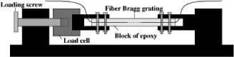
After releasing the resin block from the mould the Bragg grating has been calibrated to determine its characteristic coefficient ![]() . During the calibration operation, the Bragg grating has been submitted to uniform strains applied by the measuring apparatus sketched in Figure 4.15. Different traction loads (measured using a load cell) can be applied with a thumbscrew. An extensometer placed at the top of the resin block made it possible to calibrate the Bragg grating sensor and a
. During the calibration operation, the Bragg grating has been submitted to uniform strains applied by the measuring apparatus sketched in Figure 4.15. Different traction loads (measured using a load cell) can be applied with a thumbscrew. An extensometer placed at the top of the resin block made it possible to calibrate the Bragg grating sensor and a ![]() -value of 1.1 × 10² μ∈.mm/rad was obtained.
-value of 1.1 × 10² μ∈.mm/rad was obtained.
Once the calibration was over, we drilled two holes through the resin block, symmetrical on the two sides of the grating. The presence of these two holes causes a strain which is not uniform along the length of the block when the longitudinal tensile is applied.
Figure 4.16. Magnitude of the reflection coefficient and phase of the Bragg grating vs different traction loads
Figure 4.16a represents the magnitude of the reflection coefficient of the Bragg grating in the resin block described above, corresponding to different tensile forces. The higher the force, the more the spectrum envelope changes and shifts towards longer wavelengths. The spectrum change is a characteristic of a non-uniform strain along the Bragg grating.
Figure 4.17. Non uniform strains measured and derived from the grating phase (plain line) and simulated by finite elements (dotted line)
From the grating phase obtained under different tensile forces (see Figure 4.16b), the non-uniform longitudinal strains of the resin block are determined using relation [4.18]. These strains are represented in Figure 4.17 and it is shown that there is a good agreement between those obtained experimentally and the others obtained by finite element simulation1.
4.4.4.4. Temperature gradient measurement
The experimental system represented in Figure 4.18 has been set up to specifically create a temperature gradient along a Bragg grating introduced into a 80 mm diameter and 20 mm high PMMA block and positioned at its center. The Bragg grating we used is a 10 mm long grating with a 1.5 nm/cm chirp (variation of the period along the grating). The temperature gradient is created using an electric heater warm plate and a water cooled cold plate. Under stationary conditions, the temperature gradient obtained using this arrangement is quasi-uniform along the Bragg grating.
Figure 4.18. Apparatus for temperature gradient measurement
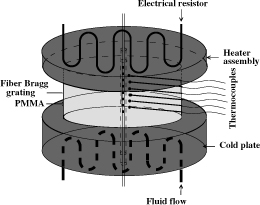
Prior to taking a temperature gradient measurement, it is necessary to calibrate the grating and determine its characteristic coefficient ![]() . For this reason, the PMMA block containing the Bragg grating has been maintained at different temperatures and a value of
. For this reason, the PMMA block containing the Bragg grating has been maintained at different temperatures and a value of ![]() has been obtained using a thermocouple.
has been obtained using a thermocouple.
In Figure 4.19a, we present the Bragg grating spectra obtained with and without the temperature gradient dotted and plain lines, respectively. Due to the changes of the chirp and the refractive index along the grating caused by the temperature gradient, the spectrum has slightly shrunk by about 160 pm and shifted toward the long wavelengths. These spectral changes depend upon the relative grating chirp and temperature gradient directions. In other words, when the grating is oriented in the other direction, the spectrum broadens.
In Figure 4.19b, we present the measurements of the phase of the Bragg grating with and without the temperature gradient dotted and plain lines, respectively. From these measurements, the temperature gradient has been determined using relation [4.18] and it is shown in Figure 4.20 to be linear with a slope of 2 °C/mm. Since the PMMA block height is 20 mm and the length of the grating we used is only 10 mm, one part only of the temperature gradient can be measured and the results
Figure 4.19. Reflection coefficient magnitude and phase of the Bragg grating without (plain line) and with (dotted line) temperature gradient
compared to those obtained using thermocouples regularly located over the whole height and inside the PMMA block. In Figure 4.20, each point corresponds to the thermocouple measurement and a very good agreement may be observed between the two results.
Figure 4.20. Temperature gradients obtained from grating phase measurements (plain line) and from thermocouples (dotted line)
4.5. Conclusion
The reflection coefficient in amplitude of a component can be measured using low coherence fiber optics interferometry which then gives access to the phase shift it causes. As far as the telecommunications are concerned, the advantage of such a measurement lies in the fact that chromatic dispersion can be derived from the phase shift that has been measured. Now this phenomenon is one of the major limiting factors for the bit rate increase. It is necessary to be able to measure it finely during the design and set up of components and transmission links. In addition, very short length samples may be characterized using interferometry. For example, one dozen centimeters is sufficient to measure the dispersion of classic fibers, with a relative precision of the order of several 10−3.
The reflection coefficient in amplitude is of prime and particular importance in the case of fibered Bragg gratings since from this spectral characterization, it is possible to realize a local characterization using an inverse method. As far as the manufacturer is concerned, this gives him the opportunity to control the inscription of the grating in real time (Espejo et al., 2004). In the field of sensors this leads us towards the measurement of profile of strains or temperature truly inside materials.
The main stake today in the field of fiber optics interferometry is the control of polarization. Some results related to this subject are to be published (Levy et al., 2006; Waagaard, 2006; Coric et al., 2006; Espejo et al., 2007). The set of feasible characterizations needs to be broadened and their precision needs to be improved. As far as the field of sensors is concerned, these measurements seemed to be highly promising. As a matter of fact, the birefringence of a fiber being bound to the shape of its cross-section, any non-isotropic crushing of the fiber induces a change in its birefringence. The local characterizations of fiber Bragg gratings, including the effects on the wave polarization, should then allow us to measure the grating deformation also in its transverse plane. We can then dispose of a three axis sensor giving access to totally new information on the constraint fields deep inside materials.
4.6. Bibliography
Broderick N. G. R., Taverner D., Richardson D. J., Ibsen M., Laming R. I., “Optical pulse compression in fiber Bragg gratings”, Physical Review Letters, vol. 79, p. 4566–4569, December, 1997.
Chapeleau X., Leduc D., Lupi C., Ny R. L., Douay M., Niay P., Boisrobert C., “Experimental synthesis of fiber Bragg gratings using optical low coherence reflectometry”, Applied Physics Letters, vol. 82, p. 4227–4229, 2003.
Chapeleau X., Leduc D., Lupi C., Boisrobert C., “Localisation et mesure d'amplitude d'un saut de phase d'un réseau de Bragg”, Journées scientifiques du CNFRS : Métrologie et Capteurs en Electromagnétisme, Meudon, 2004.
Chapeleau X., Leduc D., Lupi C., López-Gejo F., Douay M., Le Ny R., Boisrobert C., “Local characterization of fiber-Bragg gratings through combined use of low-coherence interferometry and a layer-peeling algorithm”, Applied Optics, vol. 45, p. 728–735, February, 2006.
Choma M. A., Ellerbee A. K., Yang C., Creazzo T. L., Izatt J. A., “Spectral-domain phase microscopy”, Optics Letters, vol. 30, p. 1162–1164, May, 2005.
Coric D., Limberger H. G., Salathé R. P., “Distributed measurements of fiber birefringence and diametric load using optical low-coherence reflectometry and fiber gratings”, Optics Express, vol. 14, p. 11804–11813, November, 2006.
Costa B., Mazzoni D., Puleo M., Vezzoni E., “Phase shift technique for the measurement of chromatic dispersion in optical fibers using LED's”, Journal of Quantum Electronics, vol. QE-18, no. 10, p. 1509–1515, 1982.
Delachenal N., Gianotti R., Walti R., Limberger H., Salathé R. P., “Constant high speed optical low coherence reflectometry over 0.12m scan range”, Electronics Letters, 1997.
Delachenal N., Walti R., Gianotti R., Christov S., Wagner P., Salathé R. P., Dürr U., Ulbers G., “Robust and rapid optical low-coherence reflectometer using a polygon mirror”, Optics Communications, vol. 162, no. 4–6, p. 195–199, 1999.
Desurvire E., Erbium-doped Fiber Amplifiers. Principles and Applications, Wiley Inter Science, 1994.
Dyer S., Rochford K. B., Rose A., “Fast and accurate low-coherence interferometric measurements of fiber Bragg grating dispersion and reflectance”, Optics Express, vol. 5, no. 11, p. 262–266, 1999.
Eggleton B., Mikkelsen B., Raybon G., Ahuja A., Rogers J., Westbrook P., Nielsen T., Stulz S., Dreyer K., “Tunable dispersion compensation in a 160-Gb/s TDM system by avoltage controlled chirped fiber Bragg grating”, Photonics Technology Letters, IEEE, vol. 12, no. 8, p. 1022–1024, 2000.
Eldén B., “The refractive index of air”, Metrologia, vol. 2, p. 71–80, 1966.
Espejo R. J., Svalgaard M., Dyer S. D., “Analysis of a fiber Bragg grating writing process using low-coherence interferometry and layer-peeling”, Symposium on Optical Fiber Measurements, 2004 (NIST Special Publication 1024), p. 195–198, 2004.
Espejo R. J., Dyer S. D., “Practical spatial resolution limits of high-resolution fibre Bragg grating sensors using layer peeling”, Measurement Science and Technology, vol. 18, p. 1661–1666, May, 2007.
Feced R., Zervas M., Muriel M., “An efficient inverse scattering algorithm for the design of nonuniform fiber Bragg gratings”, IEEE Journal of Quantum Electronics, vol. 35, no. 8, p. 1105–1115, 1999.
Ferdinand P., Capteurs à fibres optiques et réseaux associés , Editions Techniques et Documentation, Lavoisier, Paris, 1992.
Folkenberg J., Nielsen M., Mortensen N., Jakobsen C., Simonsen H., “Polarization maintaining large mode area photonic crystal fiber”, Optics Express, vol. 12, no. 5, p. 956–960, 2004.
Francois P. L., Monerie M., Vassallo C., Durteste Y., Alard F. R., “Three ways to implement interferential techniques: Application to measurements of chromatic dispersion, birefringence, and nonlinear susceptibilities”, Journal of Lightwave Technology, vol. 7, no. 3, p. 500–513, 1989.
Genty G., Niemi T., Ludvigsen H., “New method to improve the accuracy of group delay measurements using the phase-shift technique”, Optics Communications, vol. 204, p. 119–126, 2002.
Giaccari P., Limberger H., Salathé R., “Local coupling coefficient characterization of fiber Bragg gratings”, Optics Letters, vol. 28, no. 8, p. 598–600, 2003.
Guy M., Taylor J., Kashyap R., “Single-frequency Erbium fibre ring laser with intracavity phase-shifted fibre Bragg grating narrowband filter”, Electronics Letters, vol. 31, no. 22, p. 1924–1925, 1995.
Hill K., Fujii Y., Johnson D., Kawasaki B., “Photosensitivity in optical waveguides: application to reflection filter fabrication”, Applied Physics Letters, vol. 32, p. 647–649, 1978.
Hill K., Meltz G., “Fiber Bragg grating technology. Fundamentals and overview”, Journal of Lightwave Technology, vol. 15, no. 8, p. 1263–1276, 1997.
Jackson D. A., Ribeiro A. B. L., Reekie L., Archambault J. L., “Simple multiplexing scheme for a fiber-optic grating sensor network”, Optics Letters, vol. 18, p. 1192–1194, July, 1993.
Kashyap R., Fiber Bragg Gratings, Optics and Photonics, Academic Press, 1999.
Keren S., Rosenthal A., Horowitz M., “Measuring the structure of highly reflecting fiber Bragg gratings”, IEEE Photonics Technology Letters, vol. 15, p. 575–577, April, 2003.
Kersey A., Berkoff T., Morey W., “High-resolution fibre-grating based strain sensor with interferometric wavelength-shift detection”, Electron. Lett., vol. 28, p. 236–238, 1992.
Kersey A., “A review of recent developments in fiber optic sensor technology”, Opt. fiber Technol., vol. 2, p. 291–317, 1996.
Kersey A., Davis A., Patrick H., Leblanc M., Koo K., Askins C., Putnam A., Friebele E., “Fiber Grating Sensors”, Journal of Lightwave Technology, vol. 15, no. 8, p. 1442–1463, 1997.
Krug P., Stolte R., Ulrich R., “Measurement of index modulation along an optical fiber Bragg grating”, Optics Letters, vol. 20, no. 17, p. 1767–1769, 1995.
Leduc D., Chapeleau X., Lupi C., Le Ny R., Boisrobert C., “Accurate low-coherence interferometric relative group delay and reflectance measurements; characterization of a free space optics multiplexer/demultiplexer”, Journal of Optics A: Pure and Applied Optics, vol. 5, p. 124–128, 2003.
Leduc D., Chapeleau X., Lupi C., Gejo F. L., Douay M., Ny R. L., Boisrobert C., “Experimental synthesis of fiber Bragg gratings index profiles: comparison of two inverse scattering algorithms”, Measurement Science and Technology, vol. 18, no. 1, p. 12–18, 2007.
Leitgeb R. A., Hitzenberger C. K., Fercher A. F., “Performance of fourier domain vs. time domain optical coherence tomography”, Optics Express, vol. 11, p. 889–894, April, 2003.
Levy E. C., Horowitz M., “Layer-peeling algorithm for reconstructing the birefringence in optical emulators”, Journal of the Optical Society of America B Optical Physics, vol. 23, p. 1531–1539, August, 2006.
Lupi C., Leduc D., Goudard J. L., Ny R. L., Boisrobert C., “Fiber amplifiers: low coherence reflectometry applied to characterization of fiber homogeneity”, Proceedings of OFC 2001, 2001.
Palavicini C., Jaouën Y., Debarge G., Kerrinckx E., Quiquempois Y., Douay M., Lepers C., Obaton A.-F., Melin G., “Phase-sensitive optical low-coherence reflectometry technique applied to the characterization of photonic crystal fiber properties”, Optics Letters, vol. 30, p. 361–363, February, 2005.
Patil A., Rastogi P., “Phase measurement techniques and their applications”, Optics and Lasers in Engineering, vol. 45, p. 253–348, 2007.
Peral E., Capmany J., Marti J., “Iterative solution to the Gel'fand-Levitan-Marchenko coupled equations and application to synthesis of fiber gratings”, Journal of Quantum Electronics, vol. 32, no. 12, p. 2078–2084, 1996.
Poladian L., “Simple grating synthesis algorithm”, Optics Letters, vol. 25, no. 11, p. 787–789, 2000.
Poladian L., Ashton B., Padden W., Michie A., Marra C., “Characterization of phase-shifts in gratings fabricated by over-ditherig and simple displacement”, Optical Fiber Technology, vol. 9, p. 173–188, 2003.
Rao Y.-J., “Review article: in-fibre Bragg grating sensors”, Measurement Science and Technology, vol. 8, p. 355–375, April, 1997.
Rao Y.-J., “Recent progress in applications of in-fibre Bragg grating sensors”, Opt. Lasers Eng., vol. 31, p. 297–324, 1999.
Ritari T., Ludvigsen H., Wegmuller M., Legré M., Gisin N., Folkenberg J., Nielsen M., “Experimental study of polarization properties of highly birefringent photonic crystal fibers”, Optics Express, vol. 12, no. 24, p. 5931–5939, 2004.
Robinson D. W., Reid G. T., Interferogram Analysis, IOP Publishing, 1993.
Robinson E., “Dynamic predictive deconvolution”, Geophys. Prospecting, vol. 23, p. 779–797, 1975.
Rose A., Wang C.-M., Dyer S., “Round Robin for optical fiber Bragg grating metrology”, Journal of research of the National Institute of Standards and Technology, vol. 105, no. 6, p. 839–866, 2000.
Rosenthal A., Horowitz M., “Inverse scattering algorithm for reconstructing strongly reflecting fiber Bragg gratings”, IEEE Journal of Quantum Electronics, vol. 39, no. 8, p. 1018–1026, 2003.
Rosenthal A., Horowitz M., “Reconstruction of a fiber Bragg grating from noisy reflection data”, Optical Society of America Journal A, vol. 22, p. 84–92, January, 2005.
Sipe J., Poladian L., de Sterke C. M., “Propagation through nonuniform grating structures”, Journal of the Optical Society of America A, vol. 11, no. 4, p. 1307–1320, 1994.
Skaar J., Synthesis and characterization of fiber Bragg gratings, PhD thesis, Norwegian University of Science and Technology, 2000.
Skaar J., Wang L., Erdogan T., “On the Synthesis of Fiber Bragg Gratings by Layer Peeling”, IEEE Journal of Quantum Electronics, vol. 37, no. 2, p. 165–173, 2001.
Song G., Shin S., “Design of corrugated waveguide filters by the Gel'fand-Levitan-Marchenko inverse-scattering method”, Journal of the Optical Society of America A, vol. 2, no. 11, p. 1905–1914, 1985.
Szydlo J., Bleuler H., Wälti R., Salathè R. P., “RAPID COMMUNICATION: High-speed measurements in optical low-coherence reflectometry”, Measurement Science and Technology, vol. 9, p. 1159–1162, August, 1998.
Takada K., Kitagawa T., Hattori K., Yamada M., Horiguchi M., Hickernell R. K., “Direct dispersion measurement of highly-Erbium-doped optical amplifiers using a low coherence reflectometer coupled with dispersive Fourier spectroscopy”, Electronics Letters, vol. 28, no. 20, p. 1889–1891, 1992.
Thirstrup C., Shi Y., Baekkelund P., Palsdottir R., “Modulation of absorption and refractive index in Er3+doped fibers”, Fiber and Integrated Optics, vol. 15, no. 1, p. 1–6, 1996.
Waagaard O. H., “Polarization-resolved spatial characterization of birefringent Fiber Bragg Gratings”, Optics Express, vol. 14, p. 4221–4236, May, 2006.
Yun S. H., Tearney G. J., de Boer J. F., Iftimia N., Bouma B. E., “High-speed optical frequency-domain imaging”, Optics Express, vol. 11, p. 2953–2963, November, 2003.
1a Chapter written by Xavier CHAPELEAU, Dominique LEDUC, Cyril LUPI, Virginie GAILLARD and Christian BOISROBERT.