CHAPTER 4
IMPLICIT EULER METHOD
Some differential equations, such as stiff equations, are difficult to approximate using explicit methods because the stability condition imposes severe restrictions on the time step. It is therefore very useful to introduce a new class of methods, called implicit methods. In this chapter we explain some basic properties of stiff equations by analyzing a simple model equation. Then we introduce the implicit Euler method, which is the most basic implicit method. At the end of the chapter a very simple variable-step-size strategy is explained. This strategy shows the fundamental idea behind more complex strategies used in higher-order methods.
4.1 Stiff equations
Many applications lead to Stiff differential equations. A simple example of a stiff equation is
which can also be written as
This equation can be solved exactly using lemma 1.2. The exact solution is
To gain insight into the behavior of the solution, instead of analyzing the exact solution (4.2), we prefer to use a general procedure to obtain the dominant terms of this solution. This procedure has the advantage that it can be applied to more general problems where the exact solutions are not known.
If we formally set ε = 0 in (4.1), we see that the function y = sin(t) satisfies the equation. This motivates us to define a new variable y1 by
![]()
For the function y1 (t), one obtains
Thus, the forcing in the y1-equation is reduced to order ![]() (ε). We repeat the process and define y2 by
(ε). We repeat the process and define y2 by
![]()
Then y2 satisfies
and the forcing is of order ![]() (ε2). Clearly, we could continue the process and reduce the forcing to even higher order in ε.
(ε2). Clearly, we could continue the process and reduce the forcing to even higher order in ε.
Since the initial data in the y2-equation are ![]() (1), in general, the function y2 will not be small. Therefore, we now solve
(1), in general, the function y2 will not be small. Therefore, we now solve
![]()
that is,
![]()
Then the function r(t) = y2 (t) − b(t) solves
The function r(t) plays the role of a remainder term: The forcing and the initial data in the r-equation are both small, and therefore we can expect r(t) to be small. Indeed, using the explicit formula (1.9), we obtain
![]()
and can estimate |r(t)|,
![]()
To summarize, the solution y(t) of (4.1) has the following representation:
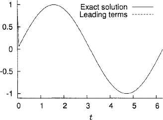
The representation (4.4) provides the leading terms of the asymptotic expansion of the exact solution y(t). It shows that except for a small remainder r(t) = ![]() (ε2), the solution of (4.3) consists of a slowly varying part, sin(t) − ε cos(t), and an initial layer, e−t/ε(y0 + ε). Figure 4.1 shows a plot of both the exact solution (4.2) and the first three terms of the asymptotic expansion (4.4) [i.e., without the remainder r(t)].
(ε2), the solution of (4.3) consists of a slowly varying part, sin(t) − ε cos(t), and an initial layer, e−t/ε(y0 + ε). Figure 4.1 shows a plot of both the exact solution (4.2) and the first three terms of the asymptotic expansion (4.4) [i.e., without the remainder r(t)].
Figure 4.1 The exact solution (4.2) and the leading terms in the asymptotic expansion (4.4) look completely superimposed in this plot.
Suppose that we try to solve (4.1) numerically by the explicit Euler method. To obtain a reasonable approximation, we must choose the step size k so that λk = −k/ε belongs to the stability region of the method (i.e., so that k ≤ 2ε). From an accuracy point of view, such a small step size is adequate in the initial layer, where the solution changes rapidly. Away from the initial layer, one would like to choose a larger step size since the solution varies slowly. With explicit Euler, however, a larger step size cannot be chosen. If k > 2ε, the method becomes unstable, which leads to growing rapid oscillations.
4.2 Implicit Euler method
When approximating the solution of (4.1), the possibility of choosing a small time step to solve the initial layer and a bigger time step for the rest of the solution can be implemented for the implicit Euler method. Assume that we want to approximate
then
Definition 4.1 The implicit Euler method to approximate (4.5) is defined by
For (4.1) the approximation reads
![]()
To discuss how the approximation behaves, we derive an asymptotic expansion for vn = vn(k,ε) which is similar to the asymptotic expansion of the exact solution y(t) given in (4.4).
First we make a change of variables,
![]()
and obtain
Here we denote by D− the difference operator
![]()
so that, by Taylor expansion,
We repeat the process and set
![]()
Then (v2)n satisfies
The equation for (v2)n can be written as
To obtain the discrete limit layer, we solve the homogeneous equation
![]()
that is,
![]()
Thus,
![]()
where
![]()
is the solution operator. Then if we define
![]()
ρn satisfies the same difference equations as (v2)n does, but the initial value is ρ0 = 0. We can now use the discrete version of Duhamel’s principle. If we identify ρn with en and the inhomogeneity in (4.7) with kRn, we can apply Lemma 2.6. We have
By Taylor expansion
![]()
so that
![]()
Therefore,
The last factor on the right-hand side is a finite geometric series [see (A.1)], so that
As ε/(ε + k) < 1, from (4.8) we have
![]()
Thus, for the complete solution vn we get
Comparing (4.9) with (4.4), we see that the slowly varying part of vn agrees with the corresponding part of the exact solution, except for terms of order ![]() (ε2). The comparison of the initial layer terms is more subtle. Here we must compare
(ε2). The comparison of the initial layer terms is more subtle. Here we must compare
with the corresponding discrete term
By Taylor expansion
![]()
Thus, if k/ε ![]() 1, the two terms (4.10) and (4.11) are close for all n = 0,1, …. On the other hand, if k/ε is not small, the two terms (4.10) and (4.11) are not close to each other for small n, and therefore vn is not a good approximation for yn in the initial layer. If k/ε is not small but n is large, terms (4.10) and (4.11) are both close to zero. This implies that vn is a good approximation for yn outside the initial layer, even if k/ε is not small.
1, the two terms (4.10) and (4.11) are close for all n = 0,1, …. On the other hand, if k/ε is not small, the two terms (4.10) and (4.11) are not close to each other for small n, and therefore vn is not a good approximation for yn in the initial layer. If k/ε is not small but n is large, terms (4.10) and (4.11) are both close to zero. This implies that vn is a good approximation for yn outside the initial layer, even if k/ε is not small.
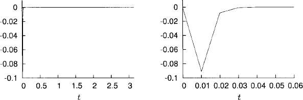
In Figure 4.2 we have plotted the error en = yn − vn for y0 = 1, ε = 10−3, k = 10−2. The exact solution was given in (4.2), while vn was computed numerically. Clearly, k/ε = 10 is not small. Nevertheless, as predicted by our analysis, away from the initial layer the error is small.
Figure 4.2 Error en = yn − vn in the interval t ![]() [0, 2π] (left plot), and of the initial layer, t
[0, 2π] (left plot), and of the initial layer, t ![]() [0,0.06], (right plot).
[0,0.06], (right plot).
We now use the truncation error analysis to discuss the error of the implicit Euler method in the more general case (4.5). We assume that Re λ ≤ 0, with |λ| not large. By definition the truncation error Rn is obtained when we substitute the exact solution y(t) in the difference equations (4.6). By Taylor expansion,
![]()
and therefore,
We can write this in the form
Let us note that, to leading order, the truncation errors for the explicit and implicit Euler methods are the same: We have Rn = (k/2)(ytt)n + ![]() (k2) in both cases. However, the stability region for the two methods is completely different. For the explicit Euler method, as we have seen in Section 2.2, the stability region consisted of all points λk in the complex plane with
(k2) in both cases. However, the stability region for the two methods is completely different. For the explicit Euler method, as we have seen in Section 2.2, the stability region consisted of all points λk in the complex plane with
![]()
that is, the stability region is a disk with radius 1 about the point −1. For the implicit Euler method the amplification factor is (1 − λk)−1, and we have
![]()
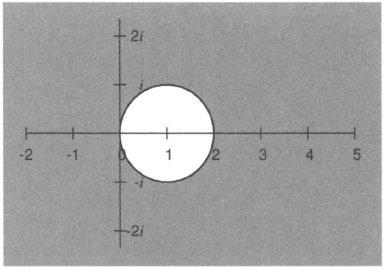
which holds if and only if |1 − λk| ≥ 1; That is, the stability region consists of all points λk in the complex plane outside the disk of radius 1 about point 1 (see Figure 4.3). In particular, all points λk with Re λ < 0 are in the stability region, no matter how large one chooses the step size k. One says that for Re λ < 0, the implicit Euler method is unconditionally stable.
Figure 4.3 The shadowed region is the stability region of the implicit Euler method.
Let us discuss the implications of this good stability property for the error en = yn − vn. Notice that (4.6) can also be written as
Subtracting (4.13) from (4.12), we obtain
By Lemma 2.6,
where
![]()
By assumption we have Re λ < 0, and therefore λk always belongs to the stability region. This yields
![]()
and the representation (4.14) implies that
To leading order, kRm ≃ (k2/2)(ytt)m, and therefore (4.15) tells us that we should choose k so that |(k2)(yt)m| is small everywhere.
What does this say for our example (4.1)? In the example we have, using (4.4),
The ![]() (k2)-term is bounded by Ck2 with C independent of ε. In the initial layer, where the term e−t/ε is
(k2)-term is bounded by Ck2 with C independent of ε. In the initial layer, where the term e−t/ε is ![]() (1), we have to choose k so that k
(1), we have to choose k so that k ![]() ε in order to make (k2/2)|ytt| small. On the other hand, outside the initial layer, where the term e−t/ε is small, it suffices to choose k
ε in order to make (k2/2)|ytt| small. On the other hand, outside the initial layer, where the term e−t/ε is small, it suffices to choose k ![]() 1. This requirement is then independent of ε. Our analysis suggests that we work with two different step sizes (see Figure 4.4): First we divide the t-axis into two intervals,
1. This requirement is then independent of ε. Our analysis suggests that we work with two different step sizes (see Figure 4.4): First we divide the t-axis into two intervals, ![]() and
and ![]() . Here
. Here
Figure 4.4 Grid with two different step sizes.
![]()
is chosen so that ε−2e−tε/ε ![]() 1. The interval 0 ≤ t ≤
1. The interval 0 ≤ t ≤ ![]() is viewed as the initial layer, because the exponential term ε2e−t/ε in (4.16) is small for t >
is viewed as the initial layer, because the exponential term ε2e−t/ε in (4.16) is small for t > ![]() . Second, in the interval 0 ≤ t ≤
. Second, in the interval 0 ≤ t ≤ ![]() , we use a step size k with k/ε
, we use a step size k with k/ε ![]() 1. In the remaining interval, t ≥
1. In the remaining interval, t ≥ ![]() , we can work with a step size k satisfying only k
, we can work with a step size k satisfying only k ![]() 1.
1.
For more complicated problems, which cannot be analyzed as easily, it is a good and common practice to use methods that regulate the step size during computations.
4.3 Simple variable-step-size strategy
Let us describe a simple strategy to construct a variable-step-size implicit Euler method. The idea is to compute, at every time step, an approximation of the leading local error term (kn2/2)(d2y/dt2)n (kn2/2)(d2y/dt2)n and to regulate the step size so as to keep this term between two given threshold values that we call M and N with 0 < M < N. More precisely, assume that vn is the computed numerical value at time tn and kn is the current step size. Then we compute the preliminary values ![]() n+1/2 and
n+1/2 and ![]() n+1 by using a step size kn/2 once and twice respectively. Using these preliminary values, we compute
n+1 by using a step size kn/2 once and twice respectively. Using these preliminary values, we compute
![]()
which is simply an approximation of the leading error term at the intermediate point tn + kn/2. Now:
![]()
![]()
![]()
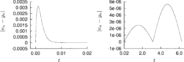
As an example we show the solution to our model problem (4.1) for t ![]() [0, 2π], with initial condition y0 = 1, obtained by applying the implicit Euler method with the variable-step-size strategy just described. The threshold values we use are M = 10−6 and N = 10−3 and an initial time step k0 = 10−2. In Figure 4.5 we plot the error |vn − yn| of the solution.
[0, 2π], with initial condition y0 = 1, obtained by applying the implicit Euler method with the variable-step-size strategy just described. The threshold values we use are M = 10−6 and N = 10−3 and an initial time step k0 = 10−2. In Figure 4.5 we plot the error |vn − yn| of the solution.
Figure 4.5 Error as a function of time. The error in the initial layer is on the left, and the error in the rest of the interval is on the right. Observe the different scales.
Exercise 4.1 Write a code that computes the solution to the example above and
Exercise 4.2 The trapezoidal rule (or method) to approximate the ordinary initial value problem
is the implicit method given by:
where, as usual, vn denotes the approximation to y(tn).