CHAPTER 3

HIGHER-ORDER METHODS

In this chapter we introduce one-step numerical methods that have been developed to compute higher-precision approximations of the exact solutions of ordinary differential equations. We introduce the second-order Taylor method, the improved Euler’s method, and a whole class of methods called Runge-Kutta methods. At the end we generalize the concepts of stability region and truncation error introduced for Euler’s method in Chapter 2.

3.1 Second-order Taylor method

To begin with, consider a differential equation

(3.1)

where F(t) is a smooth function. We want to derive a more accurate approximation than the one obtained from the explicit Euler method. If we think of the grid and the notation for grid functions introduced in Section 2.1, we have, by Taylor expansion,

(3.2)

Now we can use the differential equation to express dy/dt and d²y/dt² in terms of y, F, and dF/dt. This is obvious for dy/dt. Furthermore, the function d²y/dt² is obtained by differentiating the differential equation,

Therefore, we can write (3.2) as

where

Neglecting terms of order (k³), we obtain

(3.3)

This is an example of the second-order Taylor method. By construction, the local accuracy of the method is (k³), and the global error in a finite time interval (after integrating ≃ 1/k steps) is (k²).

It is easy to generalize the idea to an initial value problem

(3.4)

We have

and obtain

Definition 3.1 The second-order Taylor method for the initial value problem (3.4) is the one-step method given by

for n = 0, 1, 2, ….

Using higher-order Taylor expansions one can—in principle—obtain methods of a very high order of precision. A disadvantage of this approach is that the partial derivatives of f(y, t) are needed analytically. For example, the second-order Taylor method requires the calculation of ∂f/∂y and ∂f/∂t. In real situations these analytical derivatives may be difficult to obtain, the expressions obtained complicated, and the evaluation of these derivatives numerically costly, thus making the method inefficient.

It is remarkable that one can obtain higher-order methods that do not use derivatives of f(y, t), only evaluations of f itself. A simple example is given in the next section.

3.2 Improved Euler’s method

Definition 3.2 The improved Euler’s method for the initial value problem (3.4) is given by

and

(3.5)

for n = 0, 1, 2, 3, ….

In this method any time step v_n → v_n+1 is composed by two substeps, each of which requires one evaluation of f. The first substep calculates a preliminary new value _n+1 by the explicit Euler method. The second substep computes the new value v_n+1 by using v_n and _n+1.

In terms of the increment function Φ, the improved Euler’s method is obtained for

It is interesting to compare this method with the second-order Taylor method. Applying the improved Euler’s method to the example

we obtain

Comparing with (3.3), we see that the improved Euler’s method is coincident up to order k² with the second-order Taylor method. The difference between the two methods is locally of order k³.

3.3 Accuracy of the solution computed

We describe here a procedure that allows us to control the global error of our numerical approximation within a time interval of interest. Consider the initial value problem

(3.6)

where f(y, t) is a smooth function and approximate it by the explicit Euler method

We compute two solutions: solution v⁽¹⁾ using step size k and solution v⁽²⁾ using step size k/2. Both solutions satisfy the expansions (see Section A.3)

where y(t) is the exact solution of (3.6). From the second expansion and taking the difference between them, we get

which means that to leading order the error of v⁽²⁾ [i.e., the difference between v⁽²⁾ and the exact solution y(t)], equals the difference between v⁽¹⁾ and v⁽²⁾.

We can use this information in the following way. Let E denote an error tolerance, the maximum acceptable global error for our numerical approximation. We compute v⁽¹⁾(nk) and v⁽²⁾((2n)(k/2)) in the largest time interval 0 ≤ t = nk ≤ T in which

(3.7)

If the interval [0, T] does not cover the time interval in which we are interested, we redo the calculations with a smaller value of k. If, after some refinements, the estimate (3.7) holds in the interval of interest, we can expect that v⁽²⁾ approximates the true solution y with an error ≃ E.

In the following we try to analyze the process for a simple model problem. Consider the initial value problem

(3.8)

where λ ≠ −1. The exact solution is y(t) = e^−t/(1 + λ). We approximate using the Euler forward method,

(3.9)

In Chapter 2 we solved such difference equations. The solution is

(3.10)

where

with

Now suppose thaht we compute the solution of Euler’s method for time steps k and k/2 and consider the difference

where

(3.11)

Our formula for v_P(nk) yields

Therefore, for sufficiently small k,

On the other hand, the formula for v_H(t) yields

Therefore, the behavior of |Δ_H| depends on the stability characteristics of the ODE given. If the problem is stable (i.e., Re λ ≤ 0), the exponential factor is bounded by 1 at all times and we have, for sufficiently small k,

Thus, if the problem is stable, we can approximate the solution y(t) with a fixed, sufficiently small k. We can expect the error bound E to hold for all times.

If the problem is unstable (i.e., Re λ > 0), then

only. Thus the time interval in which the error bound is satisfied increases only in proportion to log_e(1/k).

Exercise 3.1 Modify the example above for the case in which the equation is stable (i.e., Re λ ≤ 0), but the forcing in the equation is exponentially divergent (i.e., e^t instead of e^−t). Can we have a bound for the global error for all times?

Exercise 3.2 Modify the argument at the beginning of this section to show that, if instead of the explicit Euler method to approximate the solution of (3.1) one uses a one-step method accurate of order p, the corresponding result can be written as follows.

For a given error tolerance E, neglecting terms of order k^p+1, if

then

where, as before, y(t) denotes the exact solution to the equation.

We present here an example that uses the global error control as described in this section. Assume that we want to solve the initial value problem

(3.12)

for t [0, 10], and we want to make sure that the global error of our solution is smaller that E = 10⁻⁴ during the entire time interval.

Assume also that we decide to approximate the solution with the improved Euler method. Then we write code that implements the improved Euler’s method for (3.12) and computes two solutions: the first solution v⁽¹⁾ using step size k and the second solution v⁽²⁾ using step size k/2. Our code stops computing either when the difference |v⁽¹⁾(nk) − v⁽²⁾ ((2n)(k/2))| reaches the value (2² − 1)E = 3E, or when t = 10. We start using the step size k = 0.1 and see that we do not reach the desired accuracy during the entire time interval of interest. We need to do two refinements, dividing the step size by 2 to reach the accuracy desired. Table 3.1 shows the results, and Figure 3.1 shows the solution v⁽²⁾ and the error for the three runs.

Table 3.1 Maximum values of |v⁽¹⁾(nk) − v⁽²⁾ ((2n)(k/2))| during computation time with improved Euler approximation of (3.12).

Exercise 3.3 Consider the initial value problem for a forced pendulum

Reducing this equation to a first-order system with variables Θ(t) and dΘ/dt, the improved Euler method reads, given the corresponding grid functions u and v, respectively

with initial data u₀ = 0, and v₀ = 0.

3.4 Runge-Kutta methods

In Section 2.1 we used Taylor expansion to construct a second-order accurate method for the ordinary differential equation

(3.13)

where f(y, t) is smooth. In principle, the procedure can be used to derive methods that have any prescribed order, no matter how high. The reason is simple. For any smooth function y(t) we can write the Taylor expansion

(3.14)

Then, if y(t) solves (3.13), we can use the differential equation (3.14) to express the time derivatives d^jy/dt^j as functions f^(j) (y, t), which are determined by f(y, t) and its partial derivatives of order smaller that or equal to j −1. For example, if we define f⁽¹⁾(y, t) = f(y, t), equation (3.13) gives

and differentiating the equation,

Therefore, we define

(3.15)

Differentiating once more, one finds that

(3.16)

and the process can be continued.

Neglecting terms of order k^p+1 in (3.14), we obtain a method that is accurate of order p.

Definition 3.3 The Taylor method of order p for equation (3.13) is given by

where the functions f^(j)(y, t) are defined as explained above.

High-order Taylor methods are extremely complicated and not often used in practice. In some applications one does not have an analytic expression of f(y, t) and then cannot compute the functions f^(j)(y, t) analytically. In other applications one does have the functions f^(j)(y, t) analytically, but their expressions are very complicated and, even worst, computationally too costly to evaluate.

It is the beauty of Runge-Kutta methods to avoid any differentiation of f(y, t). All that is required are evaluations of f(y, t) at judiciously chosen points. To make this idea clear we derive the simplest Runge-Kutta methods, which are second-order accurate, and then generalize to higher order.

Assume that y(t) is the solution of (3.13) with initial data y(t = 0) = y₀. Making f⁽¹⁾ and f⁽²⁾ explicit in (3.14), we obtain

(3.17)

The key idea is to recognize the terms in parentheses as terms of a two-variable Taylor expansion of f(y, t):

(3.18)

Choosing a = kf(y, t)/2 and b = k/2 in (3.18) and inserting into (3.17), we get

(3.19)

Thus, neglecting terms of order k³ we obtain a method that is second-order accurate and that does not require evaluations of any derivatives of f(y, t) but only two “nested” evaluations of f(y, t). This method can be written as

(3.20)

It is direct to check that the method we just obtained is simply the improved Euler’s method introduced in Section 3.2.

The procedure just described, starting at (3.17) and leading to the method (3.20), is not unique. For example, we can rewrite (3.17) as

and then, using (3.18) with a = kf(y, t) and b = k, we get

Again, neglecting terms of order k³, we get another second-order accurate method that can be written as

(3.21)

This method is known in the literature as the method of Heun.

The improved Euler method and the method of Heun are simply particular examples of Runge-Kutta methods of order 2.

Definition 3.4 Runge-Kutta methods of order 2 for the initial value problem for equation (3.13) with initial data y(t = 0) = y₀ are

where the coefficients α₁, α₂, β₂₁, and γ₂ satisfy

Runge-Kutta methods of order 2 are one-step methods that require two nested evaluations of the function f(y, t) and no evaluation of any derivative of f. The incremental function of these methods is

The four coefficients α₁, α₂, β₂₁, and γ₂ that define a particular method need to satisfy only three nonlinear algebraic equations. As seen earlier different solutions to these algebraic equations can be found, leading to different Runge-Kutta methods of order 2. The nonuniqueness of these solutions is a very important property that holds for all Runge-Kutta methods of any order. This freedom in choosing the coefficients that define a Runge-Kutta method can be exploited in various ways, such as minimizing the error for a particular equation or building embedded Runge-Kutta methods useful to control the time step to keep the error under tolerance. In Section 4.3 we present a very simple variable-step-size strategy that adjusts the time step using an estimate of the local error dominant term. More information on step size control and embedded Runge-Kutta methods is available in the literature [4, 8].

Runge-Kutta methods of order p for initial value problem (3.13) with initial data y(t = 0) = y₀ are methods of the form

where

and where the coefficients α_j, β_jk, and γ_j satisfy a set of nonlinear algebraic equations so that the method is locally accurate of order p + 1. There is no point in writing the set of equations for a general method of order p here. We would rather concentrate on important examples.

It is usual to present a particular Runge-Kutta method of order p by providing a table with the coefficients that define the method. Care should be taken since the table can be presented in different ways. A possible way is

(3.22)

For example, the improved Euler and Heun methods are given by

respectively.

By far, the Runge-Kutta method most widely used in applications is the classical fourth-order Runge-Kutta method with the table

Or explicitly,

Definition 3.5 The classical fourth-order Runge-Kutta method for the initial value problem (3.13) with initial data y(t = 0) = y₀ is

where

Exercise 3.4 Write a code that implements the classical fourth-order Runge-Kutta method to solve problem (3.12) for t [0,10]. Perform runs with time steps k = 10⁻², k/2, and k/4. Plot the solution v(t, k/4). Your code should also compute the precision quotient

Based on the solution expansion, show that Q(t) should be close to the value 2⁴ = 16 most of the time. Plot the Q(t) obtained with your code. Is the result satisfactory?

3.5 Regions of stability

Consider the initial value problem

(3.23)

The solutions v_n of all the difference approximations that we have discussed to approximate (3.23) converge, in maximum norm, to the solution y(t) for k → 0. More precisely, for any finite interval 0 ≤ t ≤ T where the exact solution y(t) exists and is smooth, we have

(3.24)

where C = C(T) is a constant independent of step size k and p is the accuracy order of the method. We have seen that p = 1 for the explicit Euler method, p = 2 for the improved Euler method, p = 4 for the classical Runge-Kutta method, and p depends on the order of expansion for Taylor’s method. As for the case of the explicit Euler method, the estimate (3.24) implies that the error converges to zero as k → 0.

We now want to generalize the idea of a stability region, introduced for Euler’s method in Chapter 2, to other one-step methods. If one applies any of the one-step difference methods that we have discussed so far to the model problem (2.10), which we repeat here for convenience:

(3.25)

one obtains

(3.26)

where Q(λk) is a polynomial in μ = λk, that depends on the method. The stability region of the method is defined by a requirement analogous to (2.12).

Definition 3.6 Assume that a one-step difference method applied to (3.25) yields (3.26). Then the stability region of the method consists of all complex numbers μ that satisfy

We compute and plot here, as an example, the stability region of the classical Runge-Kutta method. Definition 3.5 applied to model problem (3.5) gives

so that

with μ = λk. The stability region is the region in the complex μ-plane that satisfies |1 + Q(μ)| ≤ 1. If we plot this region in gray, we get Figure 3.2.

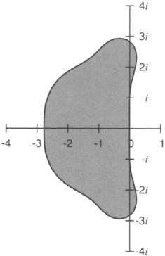
By definition, one can determine the stability region of a method by studying how the method behaves when applied to model equation (3.25). However, the stability region is of general importance: If one solves the equation dy/dt = f(y,t), one always tries to choose k so that λ_nk lies in the stability region, where λ_n = ∂f(v_n, t_n)/∂y. We discuss below why this is reasonable.

Because of its general importance, the stability region has been determined for every numerical method used in practice (see, e.g., [8]).

Exercise 3.5 Determine and plot the stability region for the improved Euler’s method.

Exercise 3.6 For the equation y = iλy, λ , determine the stability interval for the third-order method based on Taylor expansion.

Exercise 3.7 Consider the explicit Euler method applied to the equation

where λ is purely imaginary.

Find α so that the interval on the imaginary axis of the λk-plane that belongs to the stability region is as large as possible.

3.6 Accuracy and truncation error

We generalize here the concept of truncation error, introduced in Definition 2.4 for Euler’s method, to a general one-step method with increment function Φ(v, t, k).

Definition 3.7 Consider an initial value problem

and approximate it by a one-step method,

Let y(t) denote the solution of the initial value problem in some interval 0 ≤ t ≤ T and substitute y_n = y(t_n) into the difference equations. The truncation error R_n is defined as

(3.27)

If

(3.28)

the method is said to be accurate of order p.

As before, the truncation error R_n depends on the step size k and on the solution y(t), although we usually suppress this in our notation. As a rule, the accuracy order p of a method depends neither on the particular solution y(t) nor on the particular equation dy/dt = f(y, t) that one considers. However, there are exceptions to this rule. For example, explicit Euler’s method is a first-order method. However if one applies Euler’s method to the trivial equation dy/dt = 0, one obtains the exact solution. Thus, in this exceptional case, the approximation is accurate to any order.

Exercise 3.8 Derive the truncation error for

applied to the general problem

In both cases, find an explicit expression for the lower-order term of R_n in terms of f and its derivatives, and show that these methods are indeed accurate of order 2.

Exercise 3.9 Determine the truncation error for the method introduced in Exercise 3.7 (b). Is the best choice of a from the point of view of accuracy coincident with the best choice of α from the point of view of stability? [compare with your solution to exercise 3.7 (b)]. In a way similar to that used in Theorem 2.7, estimate the global error as a function of α.

3.7 Difference approximations for unstable problems

In Section 1.3 we discussed the concept of stability. A problem is called unstable if perturbations grow exponentially. A simple example is given by

We approximate it by the explicit Euler method

We cannot choose k > 0 so that kλ belongs to the stability region of the method since

In fact, there is no method for which λk belongs to its stability region for 0 < k < k₀, due to the following facts:

We have to relax our requirement that λk belongs to the stability region.

Definition 3.8 Approximate du/dt = λu, u(0) = 0, by the difference approximation

We call the approximation conditionally stable if its solution does not grow, in absolute value, faster than the solution of the differential equation, that is,

(3.29)

As an example, we consider the explicit Euler method. In this case

Since

the condition (3.29) is satisfied if |λ_I| ≤ |λ_R| and the explicit Euler is conditionally stable.