CHAPTER 2

METHOD OF EULER

Essentially all concepts introduced in Chapter 1 have their counterpart in this chapter. We introduce the simplest difference method that one can use to approximate an initial value problem. Most of the fundamental concepts needed to understand numerical approximations to differential equations follow the concepts introduced here for the method of Euler. These concepts are more complicated; therefore, one should understand the procedures for differential equations before one starts with the difference approximations. New concepts are accuracy, truncation error, and stability region. Also, a discrete version of Duhamel’s principle is discussed. General one-step methods are defined and a section is devoted to tests of correctness of a program.

2.1 Explicit Euler method

There are many methods of computing approximations to the solution of an initial value problem. The explicit Euler method,¹ which we discuss here, is the most easily understood and implemented. To describe it, let us first introduce the concepts of grid and grid function.

Starting form the initial time in our problem, say t = 0, we divide the t-axis into subintervals of length k > 0 and obtain a grid (see Figure 2.1). The endpoints t_n = nk, n = 0, 1, 2, … of the subintervals are called grid points. A grid function g_n = g(nk) is a function that is denned on the grid. The explicit Euler method for an initial value problem

will be derived below, but we start with the particular example

(2.1)

and use it for an error discussion.

For simplicity, let us assume that μ ≠ λ (i.e., we do not have a case of resonance). By Section 1.1 we know the exact solution,

(2.2)

Let us now replace (2.1) by a difference approximation. By Taylor expansion, we have for any smooth function y(t),

(2.3)

If y(t) is the solution of the differential equation (2.1), we can replace dy/dt by λy + e^μt and obtain

If we neglect the (k²) term and write v_n instead of y_n, we obtain the explicit Euler method for (2.1):

(2.4)

(2.5)

It is clear that the difference equation (2.4) can be solved recursively: Once v_n is known for some n, (2.4) can be used to calculate v_n+1, etc. Thus, (2.4) and (2.5) determine a unique grid function v_n, n = 0, 1, 2, …. It is also clear that this grid function depends on the step size k, but this is suppressed in our notation.

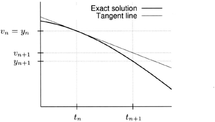
The exact solution to an initial value problem can be thought, geometrically, to be the integral curve, in the (t, y) plane, of the direction field defined by the equation that passes through the initial point (t₀, y₀). One can think of Euler’s explicit method, geometrically, as a method that computes the point (t_n+1, v_n+1) by following the tangent line to the graph of the exact solution that passes though the point (t_n, v_n) (see Figure 2.2).

It is not difficult to derive the explicit Euler method for general equations:

(2.6)

Taylor expansion gives us

Neglecting terms of order (k²), we obtain the explicit Euler method.

Definition 2.1 The explicit Euler method (or simply the Euler method) that approximates problem (2.6) is

2.2 Stability of the explicit Euler method

Consider the initial value problem

(2.7)

If one approximates this problem with Euler’s method, one expects that the difference between the approximate solution and the exact solution to (2.7) will approach zero as k → 0. However, in actual numerical computations, one might choose one or a few step sizes but cannot send k → 0. In a concrete application, how should one choose k? There are two aspects that one needs to consider to make a good choice: the stability and the accuracy of the approximation. The latter aspect is determined by the size of the truncation error.

We start the discussion of these concepts with an example. Consider the initial value problem

(2.8)

Let us approximate (2.8) by the explicit Euler method:

(2.9)

The exact solution of (2.8),

decays rapidly to zero for increasing t. On the other hand, if k > 2/100, the numerical solution v_n increases in absolute value with increasing n and does not resemble y_n at all. For the example above, a reasonable requirement is to choose k so small the the solution v_n of the difference approximation does not grow in absolute value with increasing n. Thus, one needs to choose k ≤ 2/100.

For the more general case,

(2.10)

we have the following result.

Lemma 2.2 Approximate (2.10) by the explicit Euler method:

If y₀ ≠ 0, we have

(2.11)

if and only if

(2.12)

Proof: Clearly, the solution v_n of the difference equation is given by

If |1 + λk| > 1, the absolute value of v_n grows with increasing n. On the other hand, if |1 + λk| ≤ 1, then (2.11) holds.

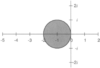
Definition 2.3 The set of all complex numbers μ = λk for which the estimate (2.12) holds is called the stability region of the explicit Euler method.

Clearly, for the explicit Euler method, the stability region consists of a closed disk with radius λk = 1 and center in λk = −1 in the complex μ = λk plane (see Figure 2.3).

2.3 Accuracy and truncation error

We start our discussion about the accuracy of the Euler approximation by defining the truncation error.

Definition 2.4 Consider the initial value problem

and approximate it by the explicit Euler method:

Let y(t) denote the solution of the initial value problem in some interval 0 ≤ t ≤ T and substitute y_n = y(t_n) into the difference equations. Then the truncation error R_n for this method is defined as

(2.13)

Remark 2.5 It is clear that the truncation error R_n depends on the step size k and on the solution y(t) under consideration. We usually suppress this in our notation.

The truncation error measures how well the solution y(t) of the differential equation satisfies the difference equations that are used to compute the numerical approximation v_n. kR_n represents the terms that we have neglected when deriving the method.

As an example, consider the initial value problem

(2.14)

for a linear equation, and approximate it by the explicit Euler method:

(2.15)

By Taylor expansion,

(2.16)

Therefore,

(2.17)

with

(2.18)

Thus, the method is first-order accurate, and for k → 0 the truncation error converges to zero. The convergence is linear with k and uniform in t; that is, as the analytic solution y(t) is smooth in a given time interval t [0, T] (in this linear example, T can be chosen as large as one pleases), we have

Thus,

and we say that the explicit Euler method is accurate of order 1.

2.4 Discrete Duhamel’s principle and global error

We now relate the stability and truncation error to the global (actual) error e_n = y_n − v_n. We start by considering the linear initial value problem of the example given in Section 2.3. Subtracting (2.15) from (2.17), we obtain

Thus, the error is determined recursively by

(2.19)

From this recursive error equation we can derive an explicit formula for the error. The result (2.21), given below, is analogous to (1.13) and constitutes an example of Duhamel’s principle for difference equations. Let

(2.20)

denote the solution operator of the homogeneous difference equations corresponding to (2.19). We have

Lemma 2.6 The solution e_n of the error equation (2.19 has, in terms of the solution operator (2.20), the representation

(2.21)

Proof: We use induction in n. For n = 1 the formula is true, because

Assuming that (2.21) holds for n, we now show its validity for n + 1. First note that

and

By (2.19) and (2.21), we have

which is the correct expression for e_n+1.

Let us now assume that Re λ < 0 in example (2.14). Then, if we choose the step size k small enough, we have |1 + λk| ≤ 1 (i.e., λk lies in the stability region of the method). Under this assumption we can estimate the error.

Theorem 2.7 Assume that λk belongs to the stability region of the method. Then the error e_n = y_n − v_n satisfies the estimate

(2.22)

Proof: First note that e₀ = 0 in (2.21). If λk belongs to the stability region, |S_k(n − 1, m)| ≤ 1, and the estimate follows from (2.21) and (2.18).

Remark 2.8 On local and global accuracy. Since a term of order (k²) has been neglected in deriving the Euler method, one says that the method is “locally accurate of order k²”, that is, if the exact solution to the equation and its Euler approximation coincide at time t, the difference between them at time t + k vanishes quadratically with k ask goes to zero. On the other hand, the global error in any finite interval is only (k) and not (k²). This is so since to get to time t ≃ 1, the right-hand side of (2.22) adds (1/k) terms of order (k²) and (k²)(1/k) = (k).

The estimate for the global error just obtained is not necessarily sharp: the best possible estimate that one can get for a linear problem. However, it has the property that one can generalize it to nonlinear problems. To see this, let us estimate the error when one approximates a nonlinear problem:

(2.23)

where the function f(y, t) is assumed to be smooth. Assume that the solution y(t) of (2.23) exists and is smooth in some time interval [0, T). Let us approximate our problem with the explicit Euler method

As above, we have for the truncation error,

Thus, the error e_n = y_n − v_n solves

By Taylor expansion,

Neglecting the quadratic terms and using the notation f_y(v_n, t_n) = λ_n, we obtain

(2.24)

The solution operator of the homogeneous equation corresponding to (2.24) is now

With this definition of S_k(n, m) the representation (2.21) of Lemma 2.6 holds. Assume now that Re λ_j < 0 [which is an assumption on df(y, t)/dy] and choose k so that λ_jk belongs to the stability region for all j. Then

and the error estimate of Theorem 2.7 also holds for the nonlinear case.

Exercise 2.1 Consider the initial value problem

with λ = −1, F(t) = sin(2πt).

and write a computer program that implements this method for using three different time-step values: k = 0.1, 0.01, 0.001. For each value of k, display the solution as a graph.

Exercise 2.2 Consider the initial value problem

(2.25)

Plot vs. k and analyze the plot for small k. Is there a linear bound for (k)? Is there a quadratic bound for (k)?

2.5 General one-step methods

The one-step methods are a large class of methods generalizing Euler’s method that approximate the initial value problem

(2.26)

and that compute the approximate solution at time t_n+1 based on the value of the approximation at t_n only.

Definition 2.9 A one-step method to approximate (2.26) is a method of the form

(2.27)

The function Φ(v, t, k) is called the increment function of the method.

The simplest choice of increment function is Φ(v, t, k) = f(v, t), leading to Euler’s explicit method.

Definition 2.10 A method (2.27) is called locally accurate of order p + 1 if

(2.28)

where y_n = y(t_n) is the exact solution y(t) of (2.26) restricted to the grid.

In other words, the method (2.27) is locally accurate of (k^p+1) if it is obtained from a relation (2.28) by neglecting a term of (k^p+1).

2.6 How to test the correctness of a program

Consider the initial value problem

(2.29)

and approximate it by the forward Euler method

At this point we want to introduce the solution expansion (for further details, see Section A.3), one can prove that

(2.30)

Here y(t) is the exact solution of (2.29) and φ₁ and φ₂ are smooth functions of t that do not depend on k.

Assume that we have written a program that carries out Euler’s method and we want to test if our program is correct. One cannot overemphasize the importance of such tests. Any experienced programmer distrusts programs and tests them over and over and, for complicated programs, finds errors even after having used them many times.

Test 1 Calculate the numerical solution for a given step size k, resulting in v⁽¹⁾ = v⁽¹⁾(t, k). Now calculate the solution again but this time with the step size k/2, resulting in the solution v⁽²⁾ = v⁽²⁾(t, k/2). By (2.30),

(2.31)

(2.32)

Therefore, the precision quotient,

(2.33)

Here we have assumed that φ₁(t) is not zero. Assume that we have calculated the solution y(t) of (2.29) analytically. Then we can evaluate Q(t) for all t = nk, n = 1, 2, … and we can test if Q(t) ~ 2. In practice, this test is rather reliable. However, it can happen that the test fails although the program is correct. This can happen for two reasons:

(a) The k used is too large and k²φ₂(t) + (k³) is of the same size as kφ₁(t). If, for example, we can neglect the terms (k³) and kφ₁ = k²φ₂, then (k/2)φ₁ = (k²/2)φ₂ and, therefore,

(2.34)

The remedy is to alter the test to accommodate smaller k.

(b) One applies the test at a point t where φ₁(t) = 0 or where |φ₁(t)| is very small. If φ₁(t) = 0 and φ₂(t) ≠ 0, we have for small k:

Therefore, one applies the test at many points t. If, Q(t) ~ 2 at most points and Q(t) > 2 at some points, one can be satisfied that the program has passed the test.

For equations more complicated than (2.29), it is often difficult to solve the initial value problem analytically. Let us explain how one proceeds in such cases. Consider the general problem

(2.35)

The function

will usually not satisfy (2.35). However, w is a solution of

(2.36)

where

We apply our program to solve the new equation (2.36) and can perform the test. An expansion of the form (2.30) is still valid if f(y, t) is a smooth function, so let us assume this fact for now. If the program solves (2.36) correctly, there is a good chance that it is still correct when we choose G(t) = 0, that is, when we solve the original equation (2.35).

Test 2 There is another way to test the program which does not require knowledge of an exact solution y(t). Besides the computations with step sizes k and k/2, we perform a third calculation with step size k/4 and determine v⁽³⁾(t, k/4). We obtain

(2.37)

Subtracting the expansions (2.32) from (2.31) and, similarly, subtracting (2.37) from (2.32), we obtain

We can now calculate

(2.38)

The new precision quotient (t) is determined completely by our numerical approximations. If (t) ~ 2, our program passes the test and has a good chance to be correct. Again, as in Test 1, one has to be careful to choose k small enough. Also, if |φ₁(t)| is very small, the test may fail at t even though the program is correct.

Exercise 2.3 Consider problem (2.29) and an approximation by any one-step method accurate of order p. Show that both precision quotients Q and defined in (2.33) and (2.38) should approximate, for small k, the value 2^p at most points.

Exercise 2.4 Following Exercise 2.1, modify your program to compute the precision quotient

where v⁽¹⁾(t) is the numerical solution computed with step size k and v⁽²⁾(t) is the solution computed with step size k/2. Show two plots of Q(t), the first computed using k = 0.01 and the second, using k = 0.001.

2.7 Extrapolation

By combining numerical solutions of a particular method, one can build a higher-order method. This technique is generally known as extrapolation.

Consider the initial value problem (2.35) as before. We can use the three computations, with step sizes k, k/2, and k/4, to improve the accuracy of our approximation. To simplify notation, let us drop the arguments in equations (2.31), (2.32), and (2.37). Then we have

(2.39)

(2.40)

(2.41)

Multiply (2.40) by 2 and then subtract (2.39) to obtain

(2.42)

Similarly, multiply (2.41) by 2 and then subtract from (2.40) to obtain

(2.43)

The last two equations say that 2v⁽²⁾ − v⁽¹⁾ and 2v⁽³⁾ − v⁽²⁾ are both order (k²) approximations to y = y(t). Furthermore, if we multiply (2.43) by 4 and then subtract (2.42), we obtain

This says that the combination

is an (k³) approximation to y = y(t).

Exercise 2.5 Define a precision quotient Q(t) for the extrapolated solution built above w(t, k) = (8v⁽³⁾ − 6v⁽²⁾ + v⁽¹⁾)/3 and show that Q(t) ≃ 2³ + (k).

¹ Also called the Euler forward method, or simply the Euler method.