CHAPTER 11

NONLINEAR PROBLEMS

In this chapter we discuss nonlinear problems. We are interested in smooth solutions. No general theory for nonlinear differential equations is available. Instead, we ask the following questions. Assume that we know a solution U for a particular set of data. Is the problem still solvable if we make small perturbations of the data? Does the solution depend continuously on the perturbation; that is, do small perturbations in the data generate small changes in the solution?

We can linearize the nonlinear equations around the known solution U and we will see that the properties of this linear system often determine the answer to the questions above.

In practice, one often solves nonlinear problems numerically without having any knowledge as to whether the differential equations have a solution. If the numerical solution is smooth in the sense that it varies slowly with respect to the mesh, we can interpolate the numerical solution. The interpolant solves a nearby problem and the solution of the original problem can be considered a perturbation of the numerically constructed solution. Therefore, the questions above are of interest.

For the sake of simplicity, in this chapter we treat initial value problems for partial differential equations with 1-periodic boundary conditions. Conclusions analogous to those derived in this chapter can be drawn for more general initial boundary value problems.

11.1 Initial value problems for ordinary differential equations

We start with a simple model problem

(11.1)

Here α, ε are real constants with 0 < ε 1. We assume also that y₀ > 0 and. calculate the solution explicitly. Introducing a new variable by

gives us

Therefore,

where

Solving for gives us

(11.2)

There are three different regimes.

The discussion above shows that the sign of α is the dominating factor determining the behavior of the solution. If α < 0, we can, for sufficiently small ε, neglect the nonlinear terms. This is also true if α = 0, provided that the time we consider is not too long.

The same type of result holds for general equations:

(11.3)

where F(y, t) denotes the nonlinear term.

We shall now solve a nonlinear equation,

(11.4)

using the forward Euler method. Let k > 0 denote the grid size and v_n = v(nk) the approximation of y on the grid. Euler’s forward method can be written as

(11.5)

We calculate v_n in some time interval 0 ≤ t ≤ T and want to decide whether the numerical solution v has anything to do with the analytic solution y.

It is well known (see, e.g., [5]) that we can interpolate the discrete grid function v by splines such that the resulting interpolant φ = Int(v) belongs to C^p(0, T) and

(11.6)

Here

where the D_k^jv_l denote the divided differences of order j. We can choose p arbitrarily. The constants K_p increase with p and are, for p ≤ 10, of moderate size. The estimate (11.6) is similar to the one for the periodic case that we derived in Theorem 9.2.

We want to show that φ(t) solves a nearby differential equation. We need

Lemma 11.1 Consider a time interval 0 ≤ t ≤ T which we cover by a grid t_n = nk, n = 1, 2, 3, …, N; Nk = T. Let F C¹ be a function with

Then

Proof: For t (0, T), there are grid points t_n, t_n+1 such that

Therefore,

and the lemma follows.

Without proof we state the following generalization.

Lemma 11.2 If F in Lemma 11.1 belongs to C^p, there is a constant C_p such that

We assume now that the interpolant φ belongs to C². Then dφ/dt − f(φ, t) C¹ and we have a bound for

We write, for arbitrary t,

(11.7)

and bound kR(t) using Lemma 11.1. For every grid point, by Taylor’s theorem,

Therefore, by Lemma 11.1, (11.7) holds with

R(t) is, essentially, the truncation error evaluated at the interpolant. If φ C^p, then R(t) C^p-2 and we have bounds for the derivative of R in terms of the divided differences of the numerical solution. Thus, if the numerical solution “looks smooth” which means that the divided differences are bounded, the interpolant solves a nearby differential equation given by (11.7).

This is as close as numerical methods can get us to the true solution. If we want to know how close we are to the true solution y(t), we have to use perturbation theory. We make the change of variables y(t) = φ(t) + k(t). By Taylor expansion, (11.4) becomes

and the problem for , equivalent to (11.4), is

(11.8)

Here g(, t) is quadratic in . As in the model problem, the behavior of the linearized problem

(11.9)

tells us how long (t) stays bounded. If the solution operator of (11.9) decays exponentially, then for sufficiently small k, (t) stays bounded for all times. On the other hand, if the solution operator grows exponentially, the blow-up can occur at t = (log(1/k)).

For complicated problems, one has no analytical knowledge of the behavior of the solution operator. Therefore, one relies on numerical perturbation calculations.

Instead of the Euler method, we could have used a higher-order method such as the fourth-order Runge-Kutta method. In that case the forcing in equation (11.7) would have been of order k⁴.

The procedure can also be used for partial differential equations, but the estimates of the derivatives of the interpolant become rather complicated.

11.2 Existence theorems for nonlinear partial differential equations

Consider the Cauchy problem for a quasilinear first-order partial differential equation

(11.10)

where

Even if we assume that all coefficients and data are smooth functions of all variables, no global existence theory is available. The only general results are of local character which can be phrased in the following way. Assume that we know that a nearby problem,

(11.11)

has a smooth solution in some time interval 0 ≤ t ≤ T. Here ε > 0 is a small constant. Can we infer that for sufficiently small ε, the original problem (11.10) has a solution in the same time interval and that |U − u| = (ε)? Using the arguments of Section 11.1, U can often, at least in principle, be obtained by interpolating a numerical solution of the problem.

The change of variables

leads to the system

(11.12)

Here P₀ denotes the linear operator that one obtains by linearizing P(x, t, , ∂/∂x) around U. A natural assumption is that the linear problem

(11.13)

is a well-posed problem. We shall now give arguments that under reasonable assumptions, this assumption guarantees that (11.12) also as a solution, provided that ε is sufficiently small. We start with an example and consider

(11.14)

Here α, ε are real constants and f, F C^∞ are real smooth functions which are 2π-periodic in x. We are interested in real solutions that are also 2π-periodic in x.

The most important tools to derive existence theorems are a priori estimates, that is, we assume that there is a smooth solution and derive estimates of u and its derivatives in terms of f and F and their derivatives. Once one has obtained these estimates, existence follows. Here we derive only a priori estimates. We refer to the literature (e.g., Chapter 4 of [7]) for a discussion of how to use them for existence theorems.

As before, u(x, t), ||u||² = (u, u) denote the L₂-scalar product and norm, here with respect to the interval 0 ≤ x ≤ 2π. Multiplying (11.14) with u and integrating gives

(11.15)

Integration by parts implies that

that is,

Therefore, (11.15) gives us

that is,

Therefore,

(11.16)

where

As in the ODE case, the sign of α determines whether the solution grows or stays bounded.

To obtain bounds for v = du/dx we differentiate (11.14) with respect to x and obtain

(11.17)

Therefore,

Since

it follows that

and

that is,

(11.18)

Since |v|_∞ cannot be estimated in terms of ||v||, we cannot use (11.18) directly to estimate v.

Differentiating (11.17) gives an equation for w = ∂²u/∂x²:

Therefore,

Since

we obtain

(11.19)

We now derive a Sobolev inequality to estimate |v|_∞ in terms of ||v||, ||w||. Let x₁, x₀ be two points with

then

Since

(11.20)

we obtain

(11.21)

and then (11.19) becomes

(11.22)

Together (11.18) and (11.22) represent a closed system of differential inequalities for ||v|| and ||w||. If we replace the inequality sign by an equality sign, we obtain a system of differential equations that maximizes the inequalities. This system is of the same form as the model problem in Section 11.1. The blow-up time, if any, depends on the sign of α and the size of |ε|.

There are no difficulties in estimating higher derivatives. They exist as long as ∂u/∂x, ∂²u/∂x² stay bounded.

The estimates above can be generalized to rather general mixed hyperbolic-parabolic systems. Consider, for example, the Cauchy problem quasilinear first-order system

(11.23)

Here are vector-valued functions with n components depending on and t.

are first-order operators with symmetric matrix coefficients that depend smoothly on all variables.

Integration by parts shows that there is a constant α such that

We have

Theorem 11.3 The system (11.23) has a smooth solution in some time interval 0 ≤ t < T; T depends on the sign of α and on f, F, and ε:

11.3 Nonlinear example: Burgers’ equation

We consider as an example the 1-periodic initial value problem for the viscous Burgers’ equation

(11.24)

Burgers’ equation is a particular case in which a rather complete analytical study can be carried out. Assume that the initial data is C^∞ smooth. It can be shown that if = 0—the inviscid Burgers’ equation—a solution exists and is C^∞ smooth only during a finite time because a shock may form. The existence time depends on the initial data. On the other hand, it can be shown that for positive the solution exists for all times. In the latter case, for well chosen initial data, a shock tends to form, but the second derivative on the right-hand side in (11.24) dissipates energy and the solution remains C^∞ smooth for all times. A detailed analysis of this equation, including energy estimates, existence, and smoothness can be found in Chapter 4 of reference [7].

Intuitively, the equation looks similar to the one-way wave equation we studied before, but now the propagation speed is the solution u itself. In a region where u > 0, the solution resembles a wave that moves to the right, whereas in a region where u > 0, the solution resembles a wave that moves to the left. If we choose

(11.25)

there is initially a positive peak at x = 1/4 and a negative peak at x = 3/4. With this initial data, Burgers’ equation will try to form a shock (diverging |∂u/∂x|) at the middle of the domain, x = 1/2, in finite time (t ≈ 0.25).

Here we want to investigate the problem (11.24), (11.25) numerically. We approximate the problem on the grid x_j = hj, h = 1/N, j . We call v_j^(h)(t) the approximation of u(x_j, t) on the grid. We approximate the first derivative by D₀ and the second derivative by D₊D₋ and integrate in time with Euler’s method using time step k = h²/2, so that the overall method becomes second-order accurate in h. Thus, we solve, with ,

(11.26)

We compute the solution v_j^(h) for three positive values of and look for the time t_max at which D₀v_j^(h) becomes maximum in absolute value (i.e., when the solution is closest to form a shock). For smaller values of we use smaller values of h, so that our code resolves well the high values of derivatives that appear. Once we find the value of t_max we compute a second and third solution using h/2 and h/4 up to that time and evaluate the precision quotient

(11.27)

to check that our code is running with correct precision order (Q_j ≃ 2² = 4), and that the values of h are small enough. We show the results in the Table 11.1 and Figure 11.1.

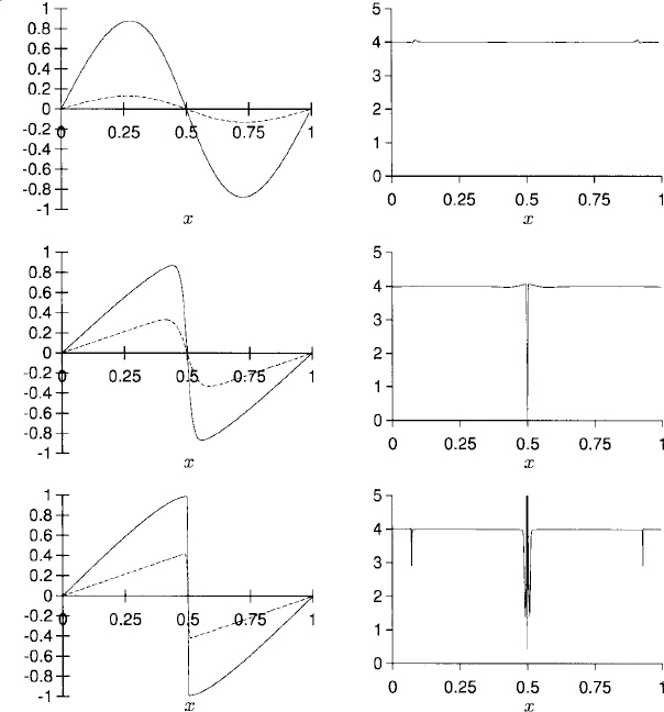
Table 11.1 Results of (11.26) for three runs with different viscosities.

It is interesting to notice in the plots of the solution that the smaller the value of , the less dissipation there is (the initial amplitude is better preserved) and the closer the solution is to develop a shock (see Figure 11.1). As time increases after t_max the energy dissipates and the amplitude decreases.

Exercise 11.1 Write a computer code to implement (11.26) and reproduce the values in Table 11.1 and the plots in Figure 11.1.