CHAPTER 1

FIRST-ORDER SCALAR EQUATIONS

In this chapter we study the basic properties of first-order scalar ordinary differential equations and their solutions. The first and larger part is devoted to linear equations and various of their basic properties, such as the principle of superposition, Duhamel’s principle, and the concept of stability. In the second part we study briefly nonlinear scalar equations, emphasizing the new behaviors that emerge, and introduce the very useful technique known as the principle of linearization. The scalar equations and their properties are crucial to an understanding of the behavior of more general differential equations.

1.1 Constant coefficient linear equations

Consider a complex function y of a real variable t. One of the simplest differential equations that y can obey is given by

(1.1)

where λ is constant. We want to solve the initial value problem, that is, we want to determine a solution for t ≥ 0 with given initial value

(1.2)

Clearly,

(1.3)

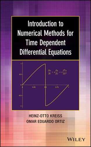
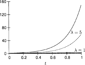
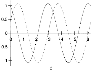
is the solution of (1.1), (1.2). Let us discuss the solution under different assumptions for the λ constant. In Figures 1.1 and 1.2 we illustrate the solution for y₀ = 1+0.4i and different values of λ.

Figure 1.1 Exponentially decaying solutions. Re y shown as solid lines and Im y as dashed lines.

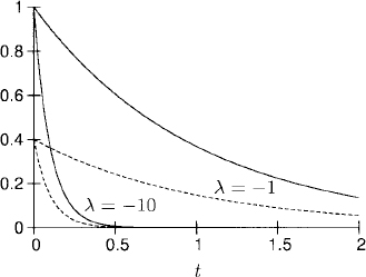
Figure 1.2 Exponentially growing solutions. Re y is shown as solid line and Im y as a dashed line.

1. λ , λ < 0. In this case both the real and imaginary parts of the solution decay exponentially. If |λ| 1, the decay is very rapid.

2. λ , λ > 0. The solution grows exponentially. The growth is slow if |λ| 1. For example, for λ = 0.01 we have, by Taylor expansion,

On the other hand, if λ 1, the solution grows very rapidly.

3. λ = i, ξ . In this case, the amplitude |y(t)| of the solution is constant in time,

If the complex initial data y₀ is written as

the solution is

which defines the real part y(t) and imaginary part y(t) of the solution. Both parts are oscillatory functions of t. The solution is highly oscillatory if |ξ| 1. Figure 1.3 shows the solution for λ = 2i and y₀ = 1 + 0.4i. Another representation of the solution is obtained if we write the initial data in amplitude-phase form,

Figure 1.3 Oscillatory solution. Re y is shown as a solid line and Im y as a dashed line.

One calls the modulus |y₀| the amplitude of y₀ and the principal argument α the phase of y₀. The solution becomes

(1.4)

The real part of the solution with λ = i, |y₀| = 1, and α = −π/4 is shown in Figure 1.4.

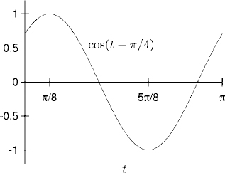
Figure 1.4 Real part of the solution (1.4).

4. The general case. Let

The solution is given by

thus,

Therefore, depending on the sign of η, the amplitude |y(t)| of the solution grows, decays, or remains constant. The phase ξt + η is a linear function of t and changes rapidly if |ξ| is large.

Next, consider the inhomogeneous problem

(1.5)

where λ, a, μ, and y₀ are complex constants. Regardless of the initial condition at first, we look for a particular solution of the form

(1.6)

Introducing (1.6) into the differential equation (1.5) gives us

that is,

If μ ≠ λ we obtain the particular solution

On the other hand, if μ = λ, the procedure above is not successful and we try to find a solution of the form¹

(1.7)

Introducing (1.7) into the differential equation gives us

The last equation is satisfied if we choose A = a; recall that λ = μ by assumption. Let us summarize our results.

Lemma 1.1 The function

is a solution of the differential equation dy/dt = λy + ae^μt.

Note that the particular solution y_P(t) does not adjust, in general, to the initial data given (i.e., y_P(0) ≠ y₀). The initial value problem (1.5) can now be solved in the following way. We introduce the dependent variable u by

Initial value problem (1.5) yields

and, since dy_P/dt = λy_P + ae^μt, we obtain

Thus, u(t) satisfies the corresponding homogeneous differential equation, and (1.3) yields

The complete solution

consists of two parts, y_P(t) and u(t). The function y_P(t) is also called the forced solution because it has essentially the same behavior as that of the forcing ae^μt. The other part, u(t), is often called the transient solution since it converges to zero for t → ∞ if Re λ < 0.

Finally, we want to show how we can solve the initial value problem

(1.8)

with a general forcing F(t). We can solve this problem by applying a procedure known as Duhamel’s principle.

1.1.1 Duhamel’s principle

Lemma 1.2 The solution of (1.8) is given by

(1.9)

Proof: Define y(t) by formula (1.9). Clearly, y(0) = y₀ (i.e., the initial condition is satisfied). Also, y(t) is a solution of the differential equation, because

This proves the lemma.

Exercise 1.1 Prove that the solution (1.9) is the unique solution of (1.8).

We shall now discuss the relation between the solution to inhomogeneous equation (1.8) and the homogeneous equation

(1.10)

We consider (1.10) with initial condition u = u(s) at a time s > 0. At a later time t ≥ s the solution is

Thus, e^λ(t-s) is a factor that connects u(t) with u(s). We will call it the solution operator and use the notation

(1.11)

The solution operator has the following properties:

(1.12)

Now we can show that the solution of inhomogeneous equation (1.8) can be expressed in terms of the solution of homogeneous equation (1.10). Then (1.9) becomes

(1.13)

In a somewhat loose way, we may consider the integral as a “sum” of many terms S(t, s_j)F(s_j)λs; think of approximating the integral by a Riemann sum. Then (1.13) expresses the solution of inhomogeneous problem (1.8) as a weighted superposition of solutions t → S(t, s) of homogeneous equation (1.10). The idea of expressing the solution of an inhomogeneous problem via solutions of the homogeneous equation is very useful. As we will see, it generalizes to systems of equations, to partial differential equations, and also to difference approximations. It is known as Duhamel’s principle.

Exercise 1.2 Use Duhamel’s principle to derive a representation for the solution of

Exercise 1.3 Consider the inhomogeneous initial value problem

where P_n(t) is a polynomial of degree n with complex coefficients. Show that the solution to the problem is of the form

where Q_m(t) is a polynomial of degree m with m = n in the nonresonance case (μ ≠ λ) and m = n + 1 in the resonance case (μ = λ). Determine ₀ in each case.

We now want to consider scalar equations with smooth variable coefficients, which leads to the next principle.

1.1.2 Principle of frozen coefficients

In many applications the problem with smooth variable coefficients can be localized, that is, it can be decomposed in many constant coefficient problems (by using a partition of unity). Then by solving all these constant coefficient problems, one can construct an approximate solution to the original variable coefficient problem. The approximation can be as good as one wants. The general theory concludes that if all relevant constant coefficient problems have a solution, the variable coefficient problem also has a solution. This procedure is known as the principle of frozen coefficients. We do not go into it more deeply here.

1.2 Variable coefficient linear equations

1.2.1 Principle of superposition

The initial value problem

(1.14)

is an example of a linear problem. It has the following properties:

To summarize, for a linear problem such as (1.14), we can use superposition of solutions to obtain new solutions. This property of linear systems, known as the superposition principle, can be used to compose solutions with complicated forcing functions out of solutions of simpler problems. Consider, for example,

(1.16)

Since

consists of three terms, we solve three problems:

We do not yet impose initial conditions, so that we can choose simple particular solutions. By Lemma 1.1, particular solutions of the equations above are

Using the superposition principle, we find that

solves

Clearly,

Therefore, the solution of (1.16) is given by

where σ is determined by the initial condition

The superposition principle relies only on linearity; it holds for any linear equation or system of linear equations, both ordinary and partial differential equations. An equation is linear if the dependent variable and its derivatives appear linearly only (i.e., as the first power), in the equation.

Exercise 1.4 Solve the initial value problem

1.2.2 Duhamel’s principle for variable coefficients

We want to discuss now the solution of problem (1.14) in terms of Duhamel’s principle. To this end we discuss the solution operator in a more abstract setting.

Consider first an initial value problem for the homogeneous equation associated with (1.14):

(1.17)

The solution operator for problem (1.17) is given by

(1.18)

Clearly,

is the solution of (1.17). With this solution operator, Duhamel’s principle [see equation (1.13)] generalizes to our variable coefficient problem (1.14):

(1.19)

This can be proved in terms of general properties of the solution operator.

It is not difficult to show that (1.18) has the following properties:

We shall use these properties to prove that (1.19) solves (1.14). Since S(0, 0) = I, we have y(0) = y₀. Also,

Therefore, y(t) given by (1.19) is the solution of (1.14).

Exercise 1.5 Find the solution operator and, using Duhamel’s principle, the solution of the following initial value problems.

1.3 Perturbations and the concept of stability

Given a problem and perturbations to it, we want to know what effect the perturbations have on the solution.

As an example, consider the initial value problem

(1.20)

with λ ≠ −1. (The exceptional case of resonance, λ = −1, can be treated with slight modifications.)

The solution of (1.20) is the decaying function

Now consider the same differential equation with perturbed initial data

(1.21)

where 0 < 1 is a small constant. Let w(t) = (t) − y(t) denote the difference between the perturbed and original solutions. Subtracting (1.20) from (1.21), we obtain

whose solution is

(1.22)

Depending on the sign of Re λ, there are three possibilities.

1. Re λ < 0. In this case the perturbation term w(t) decays exponentially with time and the solution of the perturbed problem converges to the solution of the original problem as t increases. In Figure 1.5 the solid line represents the solution with λ = −7/12, and the dashed line is the solution with perturbed initial data.

Figure 1.5 Decaying perturbation.

2. Re λ = 0. The perturbation w(t) does not decrease with time, but it does not grow either (see Figure 1.6).

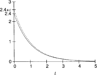
Figure 1.6 Non-decaying perturbation.

3. Re λ > 0. The perturbation grows exponentially in time. Figure 1.7 shows the perturbed and unperturbed solutions for λ = 1.

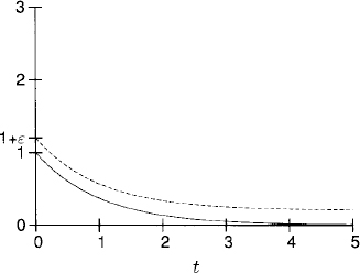
Figure 1.7 Exponentially growing perturbation.

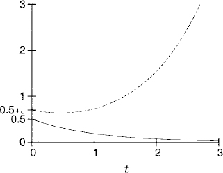
In the latter case it will be very difficult to compute the original solution accurately in long time intervals. For example, if λ = 1 and ε = 10⁻¹⁰, then

Therefore, if the calculation introduces an error ε = 10⁻¹⁰ at t = 0, this error will grow to w(T) = 1 at about T = 25. This growth holds even if no further errors, except the original error ε = 10⁻¹⁰ at t = 0, are introduced.

In applications the initial data and the forcing are never given exactly. Therefore, if Re λ > 0, one cannot guarantee that the answer computed is close to the correct answer. For Re λ < 0, the situation is the opposite: Initial errors in the data are wiped out. Problems corresponding to Re λ < 0 are called strongly stable. If Re λ = 0, the problem is stable but not strongly stable, and if Re λ > 0, the problem is unstable.

Next, let us perturb the forcing and consider

(1.23)

instead of (1.20). The error term w(t) = (t) − y(t) solves

(1.24)

and we obtain by Duhamel’s principle,

Therefore, w(t) satisfies the estimate

(1.25)

We arrive at essentially the same conclusions as those for the perturbed initial data:

There are no difficulties in generalizing this observation to linear equations with variable coefficients:

(1.26)

The influence of perturbations of the forcing and of the initial data depends on the behavior of the solution operator

Definition 1.3 Consider the linear initial value problem (1.26) and its solution operator S(t, s). The problem is called strongly stable, stable, or unstable if the solution operator satisfies, respectively, the following estimates:

where δ is a positive constant.

Exercise 1.6 Consider, instead of (1.20), the initial value problem for the resonance case

and the problem with perturbed initial data,

Show that the same conclusions of the nonresonance case can be drawn for w(t) = − y(t).

1.4 Nonlinear equations: the possibility of blow-up

Nonlinearities in the equation can produce a solution that blows up in finite time, that is, a solution that does not exist for all times. Consider, for example, the nonlinear initial value problem given by

(1.27)

For y₀ = 0 the solution is y = 0 for all times. Therefore, assume that y₀ ≠ 0 in the following. To calculate the solution, we write the differential equation in the form

and integrate:

The change of variables y(s) = v gives us

and we obtain

For y₀ > 0 the solution blows up at t = 1/y₀ (see Figure 1.8). This blow-up or divergence of the solution at a finite time is a consequence of the nonlinearity, that is, the term y² on the right-hand side of the equation. This behavior cannot occur in a linear problem. On the other hand, if y₀ < 0, the solution y(t) exists for all t ≥ 0 and converges to zero for t → ∞ (see Figure 1.9).

Figure 1.8 y₀ > 0.

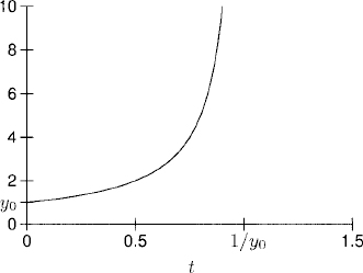
Figure 1.9 y₀ < 0.

Consider now the more general problem

(1.28)

We give here without proof a simple version of the classical existence and uniqueness theorem for scalar ordinary differential equations (see, e.g., [3], chapt. 5).

Theorem 1.4 If f(y,t) and ∂f(y,t)/∂y are continuous functions in a rectangle Ω = [y₀ − b,y₀ + b] x [t₀ − a, t₀ + a], a, b > 0, and |f(y,t)| ≤ M on Ω, there exists a unique, continuously differentiable solution y(t) to the problem (1.28) in the interval |t − t₀| ≤ Δt = min{a, b/M}.

Remark 1.5 The time interval of existence depends on how large one can choose the rectangle, and so on the initial point (y₀, t₀). The solution can be continued to the future by solving the equation with new initial conditions starting at the point (y(t₀ + Δt), t₀ + Δt). If one tries to continue the solution as much as possible, there are two possibilities:

Exercise 1.7 Show that if a smooth solution y(t) to (1.28) blows up at finite time, its derivative dy/dt blows up at the same time. Hint: Use the mean value theorem.

Exercise 1.8 Show that the converse of exercise (1.7) is false. To this end, consider the initial value problem

Explicitly find the solution y(t) and check that dy/dt → ∞ when t → (1/2)⁻ and that, nevertheless, y(t) stays bounded.

Exercise 1.9 Is it possible that the solution of the real equation

blows up at a finite time? Explain the Answer.

1.5 Principle of linearization

Consider the initial value problem

(1.29)

Assume that

A simple calculation shows that the solution of (1.29) is given by

Let ε with 0 ≤ ε 1 be a small constant and consider the perturbed problem

(1.30)

Here G(t) is a smooth function with

(1.31)

By Section 1.3 we expect that in some time interval 0 ≤ t ≤ T,

²

Therefore, we make the following change of variables:

(1.32)

Introducing (1.32) into (1.30) gives us

The form of F gives us

(1.33)

We expect that |u| ≤ 1 in some time interval 0 ≤ t ≤ T, and therefore we can neglect the quadratic term εu² to obtain the linearized equation

(1.34)

In Section 1.3 we discussed the growth behavior of the solutions of (1.34). It depends on the solution operator

Exercise 1.10 Prove, using the solution operator S(t, s), that the problem is strongly stable for λ < 0.

If the linearized equation is strongly stable (i.e., Re λ < 0), then

and, using (1.31), is bounded for all times. In this case one can also show that, for sufficiently small ε,

for all times. Thus, the linearized equation determines, to first approximation, the effect of the perturbation on the solution.

If the linearized equation is only stable, then

and

provided that

Therefore, the linearized equation describes the behavior of the perturbation in every time interval 0 ≤ t ≤ T with T²ε 1.

If the linearized equation is unstable,

and the time interval where the linearized equation (1.34) is a good approximation of (1.33) is restricted to a time interval 0 ≤ t ≤ T with

This behavior is general in nature.

Consider the nonlinear equation

(1.35)

Assume that the solution y(t) of this problem is known. Consider a perturbation

(1.36)

We make the change of variables

Since

we obtain

(1.37)

Neglecting the quadratic terms, we obtain the linearized equation

(1.38)

The effect of the perturbation depends on the stability properties of (1.38).

Linearization is a very important tool because it is used to show that the nonlinear problem has a unique solution locally.

¹The exceptional case, μ = λ, is called the case of resonance.

²From now on we frequently use the notation ; for a precise definition, consult Section A.2.