CHAPTER 10

LINEAR INITIAL BOUNDARY VALUE PROBLEMS

The purpose of this chapter is to introduce the basic ideas of initial boundary value problems for partial differential equations and their finite difference approximations. We study the model equations of Chapter 9. Energy estimates, the simplest technique to use to study well posedness for these problems, is discussed first. Then the method of lines and the energy estimates for typical semidiscrete approximations are discussed.

10.1 Well-Posed Initial Boundary Value Problems

Fourier mode analysis is not easily generalizable to problems with boundary conditions other than periodic, whereas the construction of energy estimates presents no problem. Energy estimates are thus the classical way to study well posedness of initial boundary value problems.

10.1.1 Heat equation on a strip

Here we study the initial value problem for the heat equation on a strip:

(10.1)

with either fixed Dirichlet boundary conditions, u(0, t) = U₀, u(1, t) = U₁, or homogeneous Neuman boundary conditions, ∂u(0, t)/∂x = ∂u(1, t)/∂x = 0. In the first case it is convenient to redefine the solution u(x, t) by subtracting the linear solution U₀ + x(U₁ − U₀) from it. Then the new function satisfies the same equation but with homogeneous boundary conditions. Therefore, it is sufficient to consider problem (10.1) with either

(10.2)

or

(10.3)

Smoothness of the solution. We give an example. We want to solve (10.1), (10.2) with initial data function

This initial data function is only continuous and the differential equation is not satisfied at the corners of the domain x = 0, t = 0 and x = 1, t = 0.

If we make an odd extension of f, that is,

we can calculate the exact solution of the original problem as if it were a periodic problem for x [-1, 1] using real Fourier series, as we studied before. Thus,

and the solution is

(10.4)

For t > 0 the Fourier coefficients in (10.4) decay exponentially fast with n; therefore the solution is C^∞ smooth for 0 ≤ x ≤ 1 and t > 0 even when the data were only continuous. This smoothness property generalizes to other boundary conditions and other strongly parabolic equations. Further details are provided elsewhere [7].

Energy estimate. We define the energy of the solution of the initial boundary value problem (10.1) and (10.2) or (10.3) by

(10.5)

In physical applications u(x, t) generally represents a real variable such as temperature. However, the theory can be developed for a complex u without adding any difficulty. As some of the identities we derive are useful in other problems, we treat the case of complex u(x, t).

Differentiating the energy and using the equation, we get

(10.6)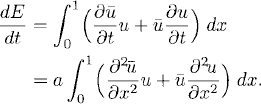

Integrating by parts, we get

(10.7)

Any of the boundary conditions (10.2) or (10.3) say that the first term on the right-hand side vanishes. The second term is nonpositive so that

(10.8)

We obtain

(10.9)

An immediate consequence of energy estimates is the uniqueness of the solution. If u₁ and u₂ are both solutions of the same initial boundary value problem (10.1) with (10.2) or (10.3), then by linearity the difference u(x, t) − u₂(x, t) is also a solution of the same problem but with vanishing initial data. Then (10.9) implies that ||u₁(·, t) − u₂(·, t)||² = 0; as the solutions are C^∞ smooth, they are the same.

General parabolic problem. Consider the more general parabolic problem on the strip 0 ≤ x ≤ 1, t ≥ 0,

(10.10)

where a > 0 and b, c , with mixed boundary conditions

(10.11)

where r₀ and r₁ are real and f is assumed to be compatible with (10.11). In this case an energy estimate of the form

(10.12)

can be shown. The energy can grow exponentially, but at a rate that is independent of the initial data. We do not give a proof of this estimate here but refer the reader to reference [6].

10.1.2 One-way wave equation on a strip

We consider here the equation

(10.13)

with initial data

(10.14)

and Dirichlet boundary conditions

(10.15)

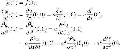
Smoothness and compatibility conditions. The smoothness of the solution of (10.13)–(10.15) depends on the smoothness of f(x), g₀(t), and g₁(t), and also on whether these functions match smoothly at the corners (0, 0) or (1,0) of the strip (i.e., the data functions satisfy the relation required by the equation at these corners).

For example, in the case a < 0, the data functions match smoothly up to second order at (0, 0) if

We give an example. We solve the problem (10.13)–(10.15) with a = 1 and

Here these two data functions are C^∞ smooth. However, g₁(t) and f(x) satisfy the equation at the right corner up to first derivatives but not to second derivatives. As a consequence, the solution

is C¹ smooth and not C² smooth for t ≥ 0.

For the solution to be C^∞ smooth, the data functions have to match at all orders at the corners. The easiest way to achieve this is to choose C^∞ smooth initial and boundary data functions so that f(x) has support on (ε, 1 − ε), 0 < ε 1, and g_i(t), i = 0, 1 vanish if t ≤ ε. By a limit process, one can generalize this data to nonvanishing data at the corners and still get a C^∞ smooth solution. Details on this procedure are available in reference [7].

Energy estimates. Let

(10.16)

We have

Lemma 10.1 If u(x, t) solves problem (10.13)–(10.15), then

with i = 0 if a < 0 and i = 1 if a > 0.

Proof: Integration by parts gives us

Then, in either case, a < 0 or a > 0, we neglect the negative term and replace u by the boundary data function in the positive term, obtaining an inequality. Integrating the inequality between 0 and t, the lemma follows.

Now, assume that the solution of (10.13)–(10.15) exists and is C^∞ smooth. One can differentiate the equation, initial data, and boundary condition as many times as one wants. For example, for a > 0,

Thus, all the derivatives satisfy the same equation as u with corresponding initial and boundary conditions. Therefore, one gets estimates for all the derivatives of u which are analogous to those for u itself. These are called a priori estimates. For example for ∂u/∂t, with a > 0, we have

In Section 10.2.4 we derive an energy estimate for a semidiscrete approximation of the problem (10.13)–(10.15). The existence and uniqueness of solution for the semidiscrete problem are not an issue. One can get estimates for all finite differences of the semidiscrete solution in analogy with the a priori estimates for the differential equation. These estimates can be obtained so that they are independent of the mesh size. Then one can prove that, in the limit when the mesh size goes to zero, the semidiscrete solution converges to a smooth function that is a solution of the differential equation. This is a way of showing the existence of solutions for the differential problem. Details on parabolic and hyperbolic equations are available in reference [7].

Exercise 10.1 Prove that the solution of (10.13)–(10.15) is unique.

10.1.3 Wave equation on a strip

In this section we study the wave equation by reducing it to a pair of one-way wave equations. Consider the initial value problem for the wave equation for φ(x, t):

(10.17)

Here c > 0 is the speed of propagation of the waves. If we consider the initial boundary value problem for 0 ≤ x ≤ 1, we need to prescribe boundary conditions. To get the correct boundary conditions, we reduce the equation to a first-order system. Defining

(10.18)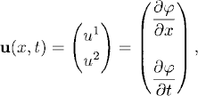

the wave equation reduces to the system

(10.19)

with

(10.20)

The matrix A is diagonable. Calculating the transformation, we get

(10.21)

Then, defining the variable

(10.22)

we obtain a diagonal system for w:

(10.23)

with initial conditions

(10.24)

The equations for w¹ and w² are decoupled one-way wave equations.

We know that we need to prescribe boundary conditions for w¹ at x = 1 and for w² at x = 0. We also want to allow coupling of the left-traveling wave with the right-traveling wave. Then the boundary conditions we consider for system (10.23) are

(10.25)

where R¹, R² are constants, and are given functions, assumed to be compatible with the initial data.

We know that the problem is well posed if R¹ = R² = 0. To see whether there are restrictions on the values of R¹, R², we study the energy inequality. Let

Following the proof of Lemma 10.1 and using the boundary conditions (10.25), we have

(10.26)

Therefore, if |R¹|, |R²| ≤ √2/2, we have the energy estimate

(10.27)

The boundary conditions (10.25) can, of course, be written in terms of the original variables using S⁻¹. We get

(10.28)

where . These conditions can be interpreted as the incoming wave prescribed in terms of the outgoing wave and a given function at each boundary.

10.2 Method of lines

In this section we study semidiscrete approximations for the model problems of Section 10.1. The differential initial boundary value problems will be reduced to systems of ordinary differential equations which can be written in matrix form. Thus, the methods we studied in the first part of the book can be used to integrate in time.

10.2.1 Heat equation

Dirichlet boundary conditions. Consider problem (10.1) with homogeneous Dirichlet boundary conditions (10.2). Let us call v_j(t) the grid function that approximates u(x_j, t) on the grid x_j = hj, j = 0, 1, 2, …, N − 1, N. We approximate the differential problem by

(10.29)

As we studied in Chapter 9, D₊D₋ is a second-order accurate approximation of the second derivative, and as the boundary conditions are exact, (10.29) is a second-order accurate approximation of the original problem.

The semidiscrete problem (10.29) is an initial value problem for a system of ODEs. It can be written in matrix form as

(10.30)

where

and

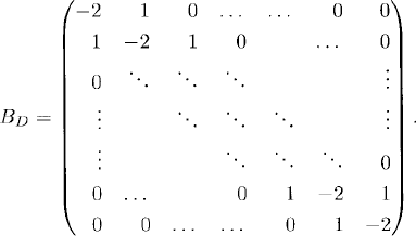
Notice that the boundary conditions v₀(t) = v_N(t) = 0 have been used for writing this matrix representation and then these two components are absent in v(t).

As B_D is real and symmetric, the system of equations (10.30) is diagonable and we can apply the theory of Chapter 6. Moreover, we will show that the eigenvalues of B_D are all negative and then system (10.30) is strongly stable as a system of ODEs.

Lemma 10.2 The matrix B_D is diagonable; its eigenvalues λ are real and lie in the interval −4 ≤ λ < 0.

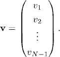
Proof: The matrix B_D is real and symmetric and is therefore diagonable with real eigenvalues. We prove that all its eigenvalues are negative by showing that B_D is negative definite. Let v be an arbitrary vector,

Then, if v^t denotes the transpose of v,

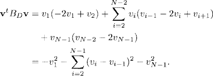
The last line is strictly negative unless v₁ = 0 and v_i = v_i-1, i = 2, 3, …, N − 1 (i.e., unless v is the zero vector). Therefore, B_D is negative definite, and all its eigenvalues are strictly negative.

We now prove that all eigenvalues of B_D are bounded in absolute value. Let λ be any eigenvalue of B_D and v one of its corresponding eigenvectors, which we assume to be normalized. Then, recalling Definition 6.1, we have

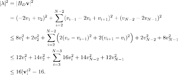
Therefore, all eigenvalues of B_D lie in the interval −4 ≤ λ < 0.

Lemma 10.2 says that (10.29) [or its matrix version, (10.30)] is strongly stable as a system of ordinary differential equations. We can use the explicit methods that we studied in the first part of the book to integrate this system in time. The restriction on the time step k follows from Lemma 10.2. For example, if we use explicit Euler, we need to choose the time step small enough that −2 ≤ kλ_j ≤ 0 for all eigenvalues λ_j of aB_D/h². By Lemma 10.2, this means that

and then we need to choose k so that

(10.31)

This is the same stability condition (CFL condition) that we found in the periodic case. Other, higher-precision methods, such as Runge-Kutta methods, are of course preferred. If we use implicit Euler method to integrate (10.30), we obtain an unconditionally stable scheme.

Exercise 10.2 Write a computer code to compute the solution of (10.29) with a = 1 and initial data function

at the same times as those of item (a).

Homogeneous Neuman boundary conditions. Consider now problem (10.1) with homogeneous Neuman boundary conditions (10.3). To be able to write a second-order accurate semidiscrete approximation, we introduce a new grid half a step displaced from the boundaries. The grid is (see Figure 10.1)

(10.32)

On this grid we study the semidiscrete approximation

(10.33)

The one-sided difference approximations D₊ and D₋ become second-order accurate at the physical boundaries x = 0 and x = 1, respectively. The values of v₀ and v_N (values of the solution at the ghost points) can be expressed in terms of v₁ and v_N-1, respectively, since the boundary conditions are equivalent to

(10.34)

The system of ODE (10.33) can be written as in (10.30), the only change being that the matrix B_D is now replaced by

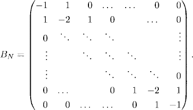
This matrix has a zero eigenvalue that corresponds to the constant solution (the correct stationary solution of this problem). With minor modifications in the proof of Lemma 10.2, it can now be proved:

Lemma 10.3 The matrix B_N is diagonable; its eigenvalues λ are real and lie in the interval −4 ≤ λ ≤ 0.

Exercise 10.3 Prove Lemma 10.3.

To integrate in time, exactly the same comments as those in the Dirichlet case hold here.

10.2.2 Finite-differences algebra

As in many semidiscrete problems, it becomes difficult to analyze whether the system of ODEs is diagonable, we use energy estimates to analyze the stability of semidiscrete problems. The algebra can be presented without any extra effort for complex grid functions.

Some basic identities. Let u_j, v_j be complex grid functions defined on any uniform grid x_j = x₀ + hj, h > 0, j . The space of such grid functions constitutes a vector space. We introduce notation for the Euclidean inner product and norm in finite-dimensional subspaces of grid functions:

(10.35)

and

(10.36)

The following identities are a direct consequence of the definitions:

(10.39)

Using these properties we can prove the discrete analog of integration by parts, generally called summation by parts.

Lemma 10.4 Let u_j, v_j be complex grid functions defined on the grid x_j = hj, j ; then

(10.40)

Proof: By the second identity in (10.38) and the first identity in (10.39), we have

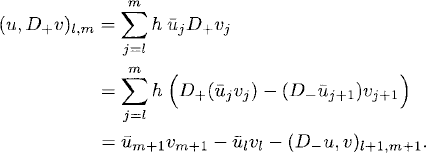
The proof of the second identity is completely analogous.

10.2.3 General parabolic problem

We study here a second-order-accurate semidiscrete approximation of the initial boundary value problem (10.10), (10.11). The semidiscrete system of equations approximating (10.10) is written on the grid (10.32):

(10.41)

The boundary conditions in (10.41) are second-order-accurate approximations of the differential boundary conditions.

As in the homogeneous Neuman case, the values of v₀ and v_N (at the ghost points) can be expressed in terms of v₁ and v_N-1, respectively, by means of the boundary conditions. We have

Choosing h small so that |hr₀| ≤ 1 and |hr₁| ≤ 1, we have

(10.42)

We want to construct the energy estimate for the semidiscrete energy:

(10.43)

We will need a bound for the grid values v_j in terms of the norm of the solution. Clearly, |v_j| ≤ h⁻¹||v||_1,N-1, but this bound is not useful because it explodes as h → 0. The useful bound involves both the norm of the grid function and the norm of its “grid derivative.” We have

Lemma 10.5 For any grid function and every ε > 0, we have

(10.44)

where C(ε) = 1 + ε⁻¹.

Proof: If f_j is constant, the lemma is trivial. Assume that f_j is not constant and let l and m be indices such that

As f_j is not constant we can assume, for simplicity, that l < m. By Lemma 10.4,

that is,

We also need a summation-by-parts formula for the centered derivative D₀.

Lemma 10.6

(10.45)

Exercise 10.4 Prove Lemma 10.6.

We can now estimate the energy (10.43). We have

(10.46)

Applying Lemmas 10.4 and 10.6 and the boundary conditions, we have

(10.47)

Using (10.42) first and then (10.44)

(10.48)

Choosing ε so that −2a + (4a(|r₀| + |r₁|) + 3|b|)ε ≤ 0, we finally have

(10.49)

where α = (4a(|r₀| + |r₁|) + 3|b|)C(ε) + 2|c| is a constant independent of h, the initial data. The energy estimate follows:

(10.50)

The semidiscrete problem behaves in the same way as the differential case (10.12); the energy can grow with time, but at a rate that is independent of the initial data. One can use explicit Euler, Runge-Kutta, implicit Euler, or the trapezoidal rule (see Exercise 4.2) to integrate in time.

10.2.4 One-way wave equation

We study here a second-order-accurate semidiscrete approximation of the problem (10.13)–(10.15). To this end we again use the grid (10.32) (see Figure 10.1), with two ghost points outside the physical boundaries. The cases a > 0 and a < 0 are completely analogous. Here we present the case a > 0.

We call v_j(t) the approximation of u(x_j, t). To have a second order accurate semidiscrete approximation, we use D₀ in the interior of the domain. Then, we need to complete the system with equations for the values at the ghost points x₀ and x_N. The value of v_N is determined at all times by the boundary condition, which is second order accurate, at x = 1. For v₀ we extend the initial data and evolution equation using the first order accurate operator D₊ so that we get a stable scheme.¹

(10.51)

In matrix form the system ODEs (10.51) becomes

(10.52)

with

Remark 10.7 The boundary data function g₁ (t) becomes the forcing for the system of ODEs. One can easily check using modern computer software, for various dimensions N, that the matrix A is diagonable and its eigenvalues have negative real part and nonzero imaginary part. The theory of Chapter 6 applies.

To prove stability of this scheme, and that the semidiscrete problem behaves as the differential problem, we construct an energy estimate. We use the energy

(10.53)

Then, using Lemma 10.6 and the boundary conditions, we have

(10.54)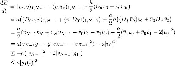

Therefore, integrating, we obtain the energy estimate

(10.55)

The semidiscrete system of ODEs behaves as the differential equation (see Lemma 10.1). To integrate in time, one needs to use a method that includes the imaginary axis in its stability region (see Remark 10.7). One can use implicit Euler or the trapezoidal rule. However, for hyperbolic equations such as ours, it is generally more efficient to use an explicit multistep method such as Adams-Bashforth.

Exercise 10.5 Consider the problem (10.13)–(10.15) with a = 1, and

Do you get a value close to 4?

10.2.5 Wave equation

To finish this chapter we present a second-order approximation to solve the initial value problem for the wave equation on a strip. Instead of approximating the problem (10.17), (10.28), we transform the problem as in Section 10.1.3 so that the problem consists in two scalar one-way wave equations coupled by the boundary conditions. Thus, all we need is a second-order semidiscrete approximation of the problem (10.23), (10.24), (10.25). We can apply the second-order approximation studied for the one-way wave equation in Section 10.2.4.

Again the grid is given by (10.32). The semidiscretized system is, calling v_jⁱ(t) the approximation of wⁱ(x_j, t), i = 0, 1,

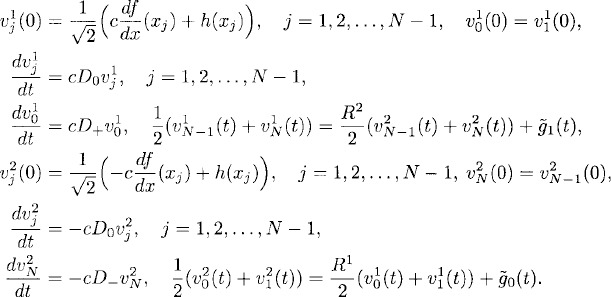
To prove the stability of this approximation, one can use the energy

(10.56)

For R¹ = R² = 0, this scheme is simply two decoupled one-way equations such as those of Section 10.2.4. Therefore, the scheme is stable. When Rⁱ, i = 0,1, are different from zero, one can get an energy estimate of the form

(10.57)

where K(t) is independent of the initial data.

Exercise 10.6 Prove (10.57).

To integrate in time, one can use the same methods mentioned in Section 10.2.4. Once the problem is solved in this varables, one can get a second-order approximation of the original function φ(x, t) of problem (10.17) since one has second-order approximations for both of its partial derivatives.

¹This is equivalent to write a second order accurate evolution for v₀ with a linearly extrapolated value of v₋₁ (i.e., h²D₊D_−v0 = 0).