Chapter 7
More About Defining Your Data
In This Chapter
![]() Understanding the special properties of dates and times
Understanding the special properties of dates and times
![]() Creating multiple response sets
Creating multiple response sets
![]() Copying variable definitions from another file
Copying variable definitions from another file
Without a definition, a number serves no purpose. For example, the number 3 could have entirely different meanings. It could be a number of miles, or an answer to a multiple-choice question, or the number of jelly beans in your pocket.
The data type is more than just a tag — it determines how the value can be manipulated. For example, date arithmetic (the distance in time between two dates) would be a nightmare to do without help. You would have to take into account leap years, and you may even have to worry about whether a day is a business day. So, it isn’t enough to merely declare that something is a date, as we do in Chapter 4. You have to make sure that the date is in the proper date format. As soon as you do that, you can take advantage of special menus for manipulating dates.
Multiple-response variables — those “check all that apply” questions on surveys — are another kind of variable type that needs extra attention. Again, when you do it properly, you can use a special menu dedicated to this type of variable. Finally, all this data definition stuff can be time consuming, so there is a special shortcut menu for copying your definition work from one dataset to another.
Working with Dates and Times
Calendar and clock arithmetic can be tricky, but SPSS can handle it all for you. Just enter the date and time in whatever format you specify, and SPSS converts those values into its internal form to do the calculations. Also, SPSS displays the date and time in your specified format, so it’s easy to read.
SPSS understands the meaning of slashes, commas, colons, blanks, and names in the dates and times you enter, so you can write the date and time almost any way you’d like. If SPSS can’t figure out what you’ve typed, it clears away what you typed and waits for you to type something again.
 Internally, SPSS keeps all dates as a positive or negative count of the number of seconds from a zero date. Here’s a bit of trivia for you. The zero date in SPSS is the birth of the Gregorian calendar in 1582. No kidding! You can choose a display format that includes or excludes the time, but the information is always there. You can even change the display format without loss of data. If the time isn’t included in the data you enter, SPSS assumes zero hours and minutes (midnight).
You determine the data type for each variable on the Data View tab of the Data Editor window. The type is chosen from the list of types shown in Figure 7-1. On the right, you select a format. SPSS uses this format to interpret your input and to format the dates for display.
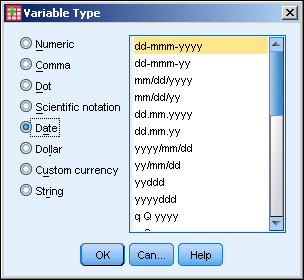
Figure 7-1: Select the data type and the format.
 SPSS uses the format you select for both reading your input and formatting the output of dates and times.
 The Columns setting of the date variable on the Variable View tab of the Data Editor window is important. The column width determines the maximum number of characters that can be displayed. If you choose a format that is too narrow to fit, the date will show up only as a row of asterisks.
The available formats are defined as a group and change according to the variable type. For example, the Dollar type has a different list of choices from those offered for the Date type.
The list of format definitions you have to choose from are constructed by combining the specifiers listed in Table 7-1. Format definitions look like mm/dd/yy and ddd:hh:mm.
Table 7-1 Specifiers in Date and Time Formats
Specifier |
Means |
dd |
A two-digit day of the month in the range 01, 02, … , 30, 31. |
ddd |
A three-digit day of the year in the range 001, 002, … , 364, 365. |
hh |
A two-digit hour of the day in the range 00, 01, … , 22, 23. |
Jan, Feb, … |
The abbreviated name of the month of the year, as in JAN, FEB, … , NOV, DEC. |
January, February, … |
The name of the month of the year, as in JANUARY, FEBRUARY, … , NOVEMBER, DECEMBER. |
mm |
When adjacent to a dd specifier in a format, a two-digit month of the year in the range 01, 02, … , 11, 12. When adjacent to an hh specifier in a format, a two-digit specifier of the minute in the range 00, 01, … , 58, 59. |
mmm |
A three-character name of a month, as in JAN, FEB, … , NOV, DEC. |
Mon, Tue, … |
The abbreviated name of the day of the week, as in MON, TUE, … , SAT, SUN. |
Monday, Tuesday, … |
The name of the day of the week, as in MONDAY, TUESDAY, … , SATURDAY, SUNDAY. |
q Q |
The quarter of the year, as in 1 Q, 2 Q, 3 Q, or 4 Q. |
Ss |
Following a colon, the number of seconds in the range 00, 01, … , 58, 59. Following a period, the number of hundredths of a second. |
ww WK |
The one- or two-digit number of the week of the year in the range 1 WK, 2 WK, … , 51 WK, 52 WK. Note: Although week numbers can be either one or two digits, the numbers always line up when printed in columns because SPSS inserts a blank in front of single-digit numbers. |
yy |
A two-digit year in the range 00, 01, … , 98, 99. The assumed first two digits of the four-digit year this represents are determined by the configuration found at Edit ⇒ Options ⇒ Data. |
yyyy |
A four-digit year in the range 0001, 0002, … , 9998, 9999. |
You can go back and change the format of a date variable at any time without fear of losing information. For example, you could enter the data under a format that accepted only the year, month, and day, and then change the format to something that contains only the hours and minutes. The format may not display all the information you entered (in fact, in this case, it won’t), but when you change the format back to something more inclusive, all your data is still there.
To enter data, choose a format — any format — that contains all the data you have. You can later change to a more limited format that displays only the information you want. But you can’t go the other way. If you later choose a format that doesn’t leave parts out, you see the defaults that were inserted by SPSS when you entered the data.
Using the Date Time Wizard
If you have dates that have been properly declared, you can easily do numerous types of calculations. Just follow these steps:
-
Open the nenana2.sav dataset.
This dataset is similar to the nenana.sav dataset except that a date time stamp has been created using the original variable, just like the demonstration in Chapter 3.
-
Choose Transform ⇒ Date and Time Wizard.
The window shown in Figure 7-2 appears.
- Select the Extract a Part of a Date or Time Variable radio button, and click Continue.
- Choose DateTime as the Date or Time variable and Day of Week as the Unit to Extract (see Figure 7-3), and click Continue.
-
Call the Result Variable the new name Day_of_Week2, and click Done.
You can check your work against Figure 7-5, if you like, but we’ll do a second calculation now. Figure 7-5 shows both calculations.
-
Return to Transform ⇒ Date and Time Wizard.
The window shown in Figure 7-2 appears again.
- Select the Calculate with Dates and Times radio button this time, and click Continue.
- Choose Current Date and Time [$TIME] as Date1 and DateTime as the Date2.
- Select the Retain Fractional Part radio button, and click Continue.
-
Call the Result Variable the new name Years_Since2, and click Finish.
The selections are shown in Figure 7-4.
- Check your work against Figure 7-5.
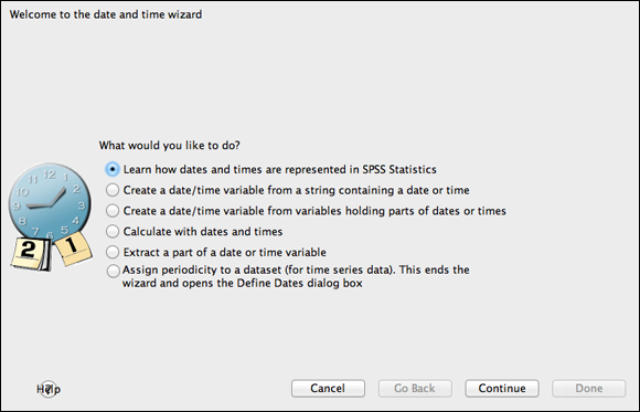
Figure 7-2: The Date and Time Wizard.
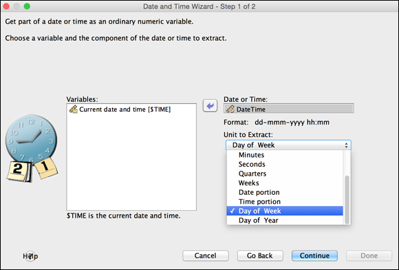
Figure 7-3: Extracting Day of Week.
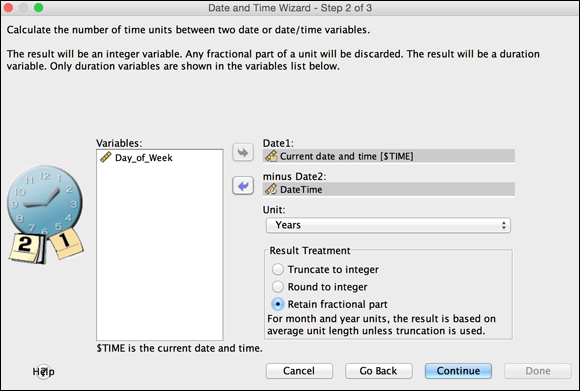
Figure 7-4: Date subtraction.
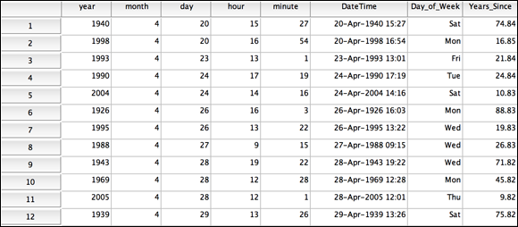
Figure 7-5: Dataset with calculations added.
Creating and Using a Multiple-Response Set
A multiple-response set is much like a new variable made of other variables you already have. A multiple-response set acts like a variable in some ways, but in other ways it doesn’t. You define it based on the variables you’ve already defined, but it doesn’t show up on the Variable View tab. It doesn’t even show up when you list your data on the Data View tab. But it does show up among the items you can choose from when defining graphs and tables.
The following steps explain how you can define a multiple-response set, but not how you can use one — that comes later when you generate a table or a graph. Also, there are two Multiple Response menus: The one in the Data menu is for tables and graphs; the one in the Analyze menu is for using special menus that you see in this example.
A multiple-response set can contain a number of variables of various types, but it must be based on two or more dichotomy variables (variables with just two values — for example, yes/no or 0/1) or two or more category variables (variables with several values — for example, country names or modes of transportation). For example, suppose you have two dichotomy variables with the value 1 defined as “no” and the value 2 defined as “yes.” You can create a multiple-response set consisting of all the cases where the answer to both is “yes,” where the answer to both is “no,” or whatever combination you want.
Do the following to create a simple multiple-response set:
-
Open the Apples and Oranges.sav dataset.
Note four dichotomous variables that have 1 for Yes and 0 for No as their possible answers, as shown in Figure 7-6.
-
Choose Analyze ⇒ Multiple Response ⇒ Define Variable Sets.
Your variables appear in the Set Definition area. If you previously defined any multiple datasets, they appear in the list on the right.
- In the Set Definition list, select each variable you want to include in your new multiple dataset, and then click the arrow to move the selections to the Variables in Set list.
- In the Variable Coding area, select the Dichotomies option and specify a Counted Value of 1.
- Select a Set Name and (optionally) a Set Label.
-
Click Add.
The new multiple-response set is created and a dollar sign ($) is placed before the name, as shown in Figure 7-7. The dollar sign in the filename identifies the variable as a multiple-response set. The new name will appear in two special menus in the Analyze menu.
There are other applications of multiple response as well, notably in the menus of the Custom Tables module, but you have to define those multiple-response sets in the Data menu. Having two menus for declaring this variable type can be a little confusing if you don’t realize this. - Click Close.
-
Choose Analyze ⇒ Multiple Response ⇒ Frequencies.
The new special variable should appear.
- Move the $Fruit variable into the Table(s) For area, as shown in Figure7-8.
-
Move the $Fruit variable into Table(s) For area.
The new special Frequencies report appears in the output window, as shown in Figure 7-9.
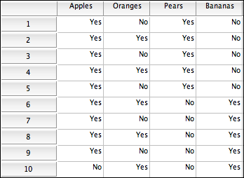
Figure 7-6: The variables are nominals with possible values of 1 and 0, which have been labeled Yes and No, respectively.
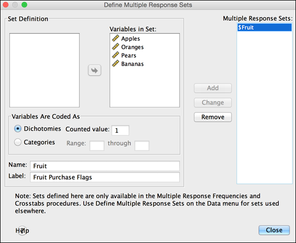
Figure 7-7: The window showing the complete definition.
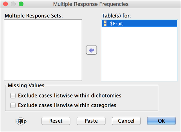
Figure 7-8: The Multiple Response Frequencies dialog box.
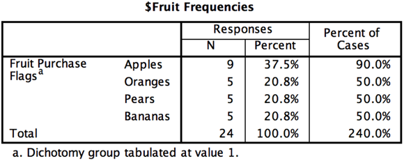
Figure 7-9: The Multiple Response Frequencies table.
This may look confusing at first, but it’s really pretty easy. Ten people bought 24 pieces of fruit. Nine pieces of fruit were apples — 37.5% of the fruit. Nine out of ten people bought apples — 90% of the people. So, the difference is the denominator: or . What makes this table special is that what you usually care about is the people with multiple responses. In other words, how many people shopping at the store are going to buy apples along with other things that they might buy? This table is the only one that easily displays them both ways.
 If multiple-response sets are a common variable type for you, you should consider trying to get the Custom Tables module because it offers lots of options for this kind of variable. You can read more about modules in Chapter 22.
Copying Data Properties
Suppose you have some data definitions in another SPSS file, and you want to copy one or more of those definitions but you don’t want the data. SPSS enables you to choose from several files and copy only the variable definitions you want into your current table.
If you have a variable of the same name defined in your table before you execute the copy, you can choose to change the existing variable definition by loading new information from another file. The copied definition simply overwrites the previous information. Otherwise, the copying procedure creates a new variable.
The following steps show you how to copy data properties:
-
Choose Data ⇒ Copy Data Properties.
The Copy Data Properties – Step 1 of 5 window, shown in Figure 7-10, appears.
- Make sure the An External SPSS Statistics Data File radio button is selected.
-
Click the Browse button, locate the file from which you want to copy variable definitions, and then click Open
The name of the selected file appears next to the Browse button.
- Click Next.
-
Select the variables you want.
Figure 7-11 displays the variable names that match in the source and destination. In the example, all three are selected, but you can turn the selection of each one on and off. Just put the mouse pointer on the one you want to select or deselect, hold down the Ctrl key, and click.
-
To use the variables you’ve selected, click Next.
If you want to copy the complete definitions of all the variables you’ve selected and completely overwrite what you have, you can click Finish. Clicking the Next button, as in this example, allows you to be more specific about which parts of the variable definitions you want to copy.
-
Choose the properties of the existing variable definitions that you want to copy to the variables you’re modifying.
In Figure 7-12, everything is selected by default, but you can skip any parts you don’t want by deselecting them. These selections apply to all variables you’ve chosen. If you want to handle each variable separately, you’ll have to run through this entire procedure again for each one, selecting different variables each time.
-
Click Next to be able to select from a list of variable properties.
If you’re satisfied with your choices, you can click Finish to complete the process. Clicking Next, as in this example, makes it possible for you to select from a list of available properties to be copied.
-
Choose any properties made available in the dialog box shown in Figure 7-13.
Depending on the variable type, different properties are available to be copied. As shown in Figure 7-13, the properties not available appear grayed out. By default, none of them is selected.
-
Click Next to move to the final dialog box.
As shown in Figure 7-14, the screen displays the number of existing variable definitions to be changed, the number of new variables to be created, and the number of other properties that will be copied. You can elect to have the action take place immediately or have the set of instructions saved as a Command Syntax script so you can execute them later. (Part VII describes using the Syntax language.)
-
Decide whether to execute the commands now or later.
You can click Finish to have the copy procedure execute immediately.
- Click Finish.
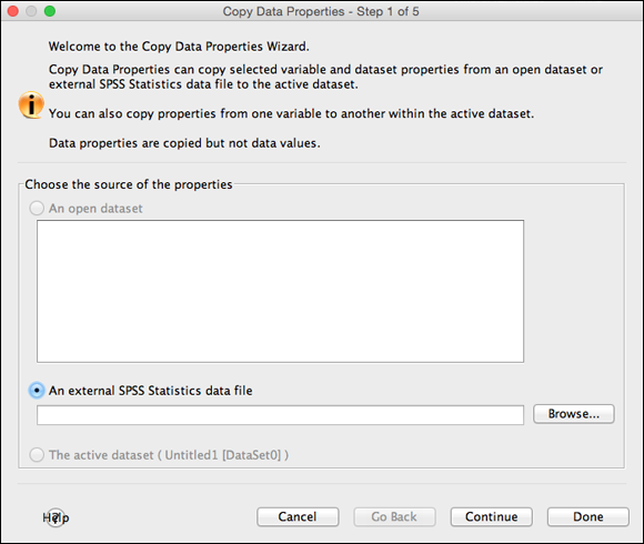
Figure 7-10: Select the file you want to use as the source of variable definitions.
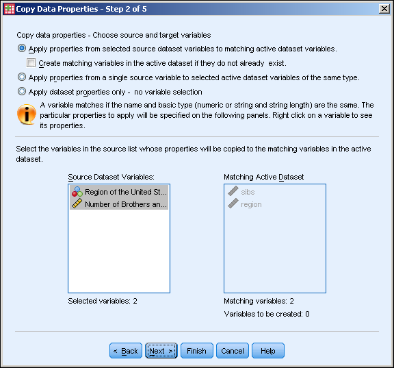
Figure 7-11: Select the source variable names you want to use for definitions.
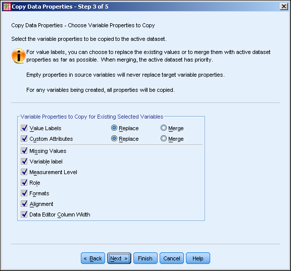
Figure 7-12: Select which attributes you want to copy.
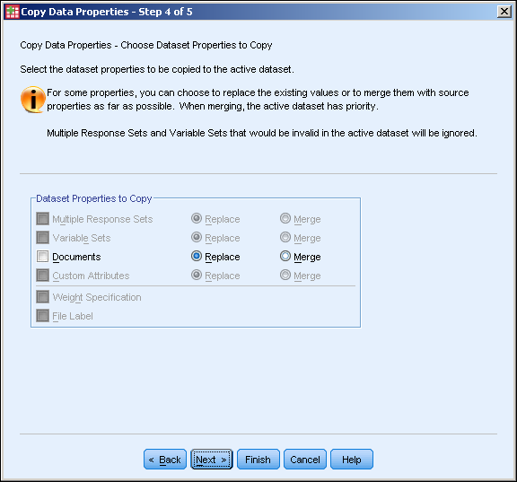
Figure 7-13: Attributes other than variable definitions can be copied from the source.
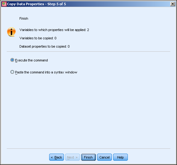
Figure 7-14: Choose to execute the commands or save the commands for later execution.
Using the basic variable types and the property descriptions you can add, you should be able to concoct any type of variable you need.