
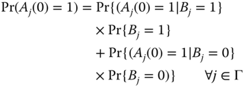
19
Cyber‐Security and Resiliency of Transportation and Power Systems in Smart Cities
Seyedamirabbas Mousavian1, Melike Erol‐Kantarci2 and Hussein T. Mouftah2
1 School of Business, Clarkson University, Potsdam, NY, USA
2 School of Electrical Engineering and Computer Science (EECS), University of Ottawa, Ottawa, ON, Canada
19.1 Introduction
A recent report from the University of Cambridge, Centre for Risk Studies and the Lloyd's of London insurance market discusses a severe attack scenario that is capable of leaving 9.3 million people in New York City and Washington, DC, without power, causing $1 trillion loss in the U.S. economy and in Lloyd's (2015). According to FireEye Inc.'s attack map in Fireeye (2012), globally over 25,000 attacks are detected in a day, and among these attacks, the energy sector is the third‐top targeted industry. Again, according to IOActive Lab's report by Cerrudu (2015), smart cities are open to cyberattacks, as well.
A cyberattack can be launched from any component of the power and electric transportation system (PETS) including a meter, phasor measurement unit (PMU), electric vehicle, or a relay. An infectious attack can propagate further in PETS and infect critical components, utility computers, and system operator servers. Considering the vast number of connected devices in the electric power system, the attack can affect a large number of devices. Hence, numerous automation and communication devices are used to measure, monitor, and control these power grid components (DoE, 2009). Ensuring all are healthy and non‐compromised is highly challenging.
It is well known that traditional boundary protection techniques are no longer effective in the energy sector (DoE, 2012). With the integration of information and communication technologies (ICT), attacks have become more permeable. In addition, with the adoption of electric vehicles, transportation is also relying on the availability of the power grid. An outage in the power grid will also incapacitate electric transportation, or malware from an electric vehicle can penetrate to the electric vehicle supply equipment (EVSE) or the so‐called charging station and can make its way into utility servers and power grid components (Caryl et al., 2013).
Previous research on cybersecurity of the smart grid focuses mostly on local attacks such as jamming, denial of service (DoS), controller malfunction, and load alteration attacks that compromise only several components of the grid. Although their local impact is not to be underestimated, if those attack behaviors are replicated, and attackers infect other components, the power grid will experience failure or malfunctioning at multiple components. In the interdependent PETS, the mobility of electric vehicles will contribute to the risk of cyberattack spread from one utility service area to the others. This implies that legacy protection techniques that rely on quarantining a set of components cannot cope with the complex spreading pattern of infectious cyberattacks on PETS.
Smart grid cybersecurity and resilience have received significant attention in recent years. There are several works on smart grid protection as well as EVI protection. In Mousavian et al. (2014), a malware‐oriented attack toward PMUs has been investigated. The PMUs have been assumed to be connected to the independent system operator (ISO) via a multi‐hop network of routers. A MILP‐based response model has been proposed in order to prevent worms from spreading. This work has been extended to address attacks in EV integration in Mousavian et al. (2015).
In Li et al. (2012), attacks on dynamic electricity pricing have been considered and their effect on EV charging has been discussed. It has been shown that price information attacks affects the optimality of EV schedules, thus leading to discrepancy between real and expected costs of EV charging. Malware on EVI can easily deploy price information attacks or load alteration attacks that may cause suboptimal schedules for EVs or incorrect pricing for utilities and customers.
In Carryl et al. (2013), the authors claim that malware infections can affect upstream equipment in the smart grid. This includes EVSEs, circuit breakers, transformers, PMUs, utility computers, and so on. Security certificates are potential solutions; however, they can be stolen via a Trojan software, and malicious users can easily sign malware as legitimate software. Therefore, having a response model for such attacks is vital for the resilience of the smart grid.
Worm propagation has been studied in the context of vehicular ad hoc networks (VANETs) where vehicles communicate safety and entertainment purposes. Khayam et al. (2004) uses the so‐called susceptible, infected, removed (SIR) model to analyze worm propagation among vehicles. The authors consider the effect of traffic density, channel fading conditions, and mobility models. In VANETs, interactive patching has been shown to better handle worm outbreaks in comparison to preemptive patching. In Mickens et al. (2005), contrary to Khayam et al. ( 2004), the SIR model has been avoided due to its inaccuracy in mobile environments, and a new model based on probabilistic queuing has been proposed.
In this chapter, we will introduce an attack‐and‐response model for EVI in the smart city. We estimate the threat level in the EVI based on charging duration. Then, we develop a protection scheme that responds to the attack by temporarily isolating compromised EVSEs. Our mixed integer linear programming (MILP) model computes the minimal number of EVSEs to be isolated to keep the desired level of service, while protecting the grid from attack propagation. We do not include EVSE‐to‐EVSE communications as most EVI applications do not require peers to communicate.
19.2 EV Infrastructure and Smart Grid Integration
The smart grid and electric vehicles are among the main drivers of the IoT, as they form a large connected network of things, such as vehicles, charging stations, smart meters, intelligent electronic devices (IED), phasor measurement units (PMU), and so on. They are also anticipated to be the drivers of green smart cities by enabling efficient integration of renewable energy and lower emissions (Northfield, 2016; Khatoun et al., 2017; Zhang et al., 2017). EVs have many advantages including reducing the nation's dependency on fossil fuels, having lower operating costs than combustion engine vehicles, and having near zero emission. They are considered as the mobile portion of the smart grid (Lopes et al., 2011; Su et al., 2012). The energy stored in EV batteries can be used as short‐term or emergency power supply for homes and businesses, in addition to supplying the motor force to drive the vehicle. Using smart grid communications through utility and service provider networks, EVs can participate in more advanced applications such as providing ancillary services. Ancillary services are operated at the background in the day‐to‐day operation of the power grid, and they include peak power supply, spinning reserves, and regulation. Despite numerous advantages and the opportunities that come with EVs, they may pose significant threats to the grid and risk the resilience of the smart grid.
EVs and EVSE, aka charging stations, which are EV's connection points to the power grid, form the EVI. An EV connect to an EVSE via an SAE 1772 connector, which can provide AC or DC power depending on the type of EVSE. Commercially Level‐1, Level‐2, and fast‐charging stations are available, in addition to wireless chargers in demo stage. The SAE 1772 connector is designed with a pilot communication line while most EVSE's have wireless access either using the IEEE 802.15.4 standard (Zigbee) or IEEE 802.11 (WiFi; Mouftah and Erol‐Kantarci, 2012; Niyato et al., 2014). National Renewable Energy Lab (NREL) has also done tests to use power‐line communications (PLC) over J1772 (Simpson et al., 2012). Communication technologies are used to exchange information between EVs and EVSEs, such as state of charge (SoC), desired charging duration, and top up amount in dollars, or distance to next destination from EVs to EVSEs, electricity price, and load control signals from EVSEs to EVs. The communication infrastructure that links EVs with EVSEs provides means to exchange such basic information. In the near future, this communication infrastructure may also be used for communicating much more information such as exchanging energy‐trading bids (Mets et al., 2010; Clement et al., 2009; Sortomme, 2011; Erol‐Kantarci et al., 2011).
Physical security, cybersecurity, and the resilience of the power grid may be at risk if the attackers launch attacks from EVs or EVSEs. Physical tampering, malicious software uploads, and load alteration are among the possible attacks on the EVI. The effects of such attacks can be as harsh as regional blackouts or a less severe but still undesirable disruption of the ISO/RTO market systems. More importantly, cyberattacks initiating from the EVI can propagate very fast with the help of the ubiquitous communications and mobility of EVs. Malware loaded to an EVSE can compromise an EV easily, and the worms can be carried around a city and its interconnections, as an EV travels and charges its battery from several other EVSEs on the road. Those malware can compromise other equipment in the smart grid, including PMUs, line and transformer monitoring and protection equipment, and smart meters. The cyber‐component of the modernized power grid makes attack propagation much more impactful than the legacy grid (Amin et al., 2015; Fang et al., 2012). Previous studies focus on protecting the smart grid equipment from malware and other potential threats (Mousavian et al., 2014; Yan et al., 2012; Amin et al., 2012) while the most vulnerable part of the grid, i.e., EVI, has been less explored. An attack scenario has been identified in Chan et al. (2013), which uses the EVI to attack the smart grid. In the scenario, the EV passes the challenge‐response authentication using the trusted computing base (TCB); however, instead of an EV, a malicious load is physically connected (plugged‐in) to the grid. The malicious load does not respond to the demand‐response commands and does not curtail its load, which triggers circuit breakers when multiple loads acts simultaneously. Thus, the mismatch between the physically connected device and the cyber‐authenticated EV risks the resilience of the smart grid. Chan (2014) proposes using two‐step challenge response to mitigate such attacks; one over the wireless communication link and another through the SEA J1772 connector. In a system where EVSEs are interconnected and EVs communicate through VANETs, EVSE2EVSE communications and EV2EV communications magnify the scale of the attacks. We consider malware spread from EV to EVSE and EVSE to EV, but the proposed response model can be easily generalized for a fully connected EVI.
19.3 System Model
19.3.1 Model Definition and Assumptions
We consider an ecosystem of EVs and EVSEs where EVs are connected to EVSEs in one hop either using wireless communications or wireline communications, which are discussed in the next section. Here, ![]() denotes the set of EVSEs and
denotes the set of EVSEs and ![]() denotes the set of detected compromised EVSEs where
denotes the set of detected compromised EVSEs where ![]() and
and ![]() . The set of EVs that have been connected to the detected compromised EVSE is given by
. The set of EVs that have been connected to the detected compromised EVSE is given by ![]() . When an EV is connected to a compromised EVSE for charging, the worm spreads from the EVSE to the EV with probability
. When an EV is connected to a compromised EVSE for charging, the worm spreads from the EVSE to the EV with probability ![]() . We assume infections are detected with a delay of
. We assume infections are detected with a delay of ![]() . The likelihood of an EVSE or an EV being compromised is referred to as threat level. The proposed protection scheme relies on a response model that minimizes the maximum threat level of all connected EVSEs at the time of detection, which is denoted by
. The likelihood of an EVSE or an EV being compromised is referred to as threat level. The proposed protection scheme relies on a response model that minimizes the maximum threat level of all connected EVSEs at the time of detection, which is denoted by ![]() . Then, compromised EVSEs are isolated temporarily while keeping the EV network operational for a load of
. Then, compromised EVSEs are isolated temporarily while keeping the EV network operational for a load of ![]() that is the forecast demand for EV charging stations. The summary of notations used throughout the next section is given in Table 19.1.
that is the forecast demand for EV charging stations. The summary of notations used throughout the next section is given in Table 19.1.
Table 19.1 Summary of notations.
| Notation | Definition |
|
|
Set of EVSEs |
|
|
Set of detected compromised EVSEs |
|
|
Set of EVs that have been connected to the detected compromised EVSE |
|
|
Number of detected compromised EVSEs |
|
|
Forecast demand for EV charging stations |
|
|
Binary decision variable which equals 1 if |
|
|
random variable which equals 1 if |
|
|
Random variable which equals 1 if |
|
|
The probability that an attack propagates from an EVSE to an EV or vice versa |
|
|
The probability of an EVSE being compromised |
|
|
the probability of an EV being compromised |
|
|
Threshold value for an operational EVI |
|
|
Number of charging stations at |
|
|
Maximum threat level of EVSEs |
19.4 Estimating the Threat Levels in the EVSE Network
In this chapter, we study the threat levels of the EVSEs when the network is experiencing an attack. We estimate the threat levels of the uncompromised EVSEs when one or more EVSEs were detected as compromised. Let us assume at time ![]() ,
, ![]() EVSEs are detected to be compromised while the remaining EVSEs are uncompromised. It takes time
EVSEs are detected to be compromised while the remaining EVSEs are uncompromised. It takes time ![]() for the cyberattack to be detected. Hence, all EVs connected to the detected compromised EVSEs during time interval
for the cyberattack to be detected. Hence, all EVs connected to the detected compromised EVSEs during time interval ![]() are likely to be compromised. During this time, there is a chance that the attack could have been propagated to uncompromised EVSEs by the compromised EVs recharging at different stations. Moreover, these new compromised EVSEs can further infect other EVs, and so forth. We represent by the probabilities,
are likely to be compromised. During this time, there is a chance that the attack could have been propagated to uncompromised EVSEs by the compromised EVs recharging at different stations. Moreover, these new compromised EVSEs can further infect other EVs, and so forth. We represent by the probabilities, ![]() and
and ![]() , the likelihood of an EVSE and an EV being compromised (also called threat level) at time
, the likelihood of an EVSE and an EV being compromised (also called threat level) at time ![]() , respectively. The initial threat levels of the EVSEs,
, respectively. The initial threat levels of the EVSEs, ![]() , are given as follows.
, are given as follows.
First, we calculate the initial threat levels of EVs, ![]() , connected to the compromised EVSE during time
, connected to the compromised EVSE during time ![]() , given that one of these EVs had infected the EVSE in the first place. We represent the number of EVs connected to the compromised EVSE during this time period by
, given that one of these EVs had infected the EVSE in the first place. We represent the number of EVs connected to the compromised EVSE during this time period by ![]() .
.
Therefore, we obtain equation (19.5) where ![]() is the probability that a cyberattack propagates from an EVSE to an EV and vice versa. Probabilistic malware spread models assume attacks propagate within the network of nodes with some probability [7]; in this paper, we adopt a similar approach.
is the probability that a cyberattack propagates from an EVSE to an EV and vice versa. Probabilistic malware spread models assume attacks propagate within the network of nodes with some probability [7]; in this paper, we adopt a similar approach.
Since all parameters in equation ( 19.5) are constant, we represent the initial threat levels by ![]() for simplicity. The infected EVs are likely to compromise the other EVSEs. To calculate the threat levels of EVSEs at time
for simplicity. The infected EVs are likely to compromise the other EVSEs. To calculate the threat levels of EVSEs at time ![]() , we need to sort EVs based on their time of connection to the EVSEs in time interval
, we need to sort EVs based on their time of connection to the EVSEs in time interval ![]() . Hence, we represent their time of connection to EVSEs by cardinal numbers for simplicity. We use equation (19.6) to calculate the threat level of an EV after getting connected to a compromised or likely compromised EVSE.
. Hence, we represent their time of connection to EVSEs by cardinal numbers for simplicity. We use equation (19.6) to calculate the threat level of an EV after getting connected to a compromised or likely compromised EVSE.
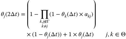
In equation ( 19.6), the first bracket represents the probability that the EV has not been compromised before connection to the EVSE; the second bracket represents the probability that the attack has not been propagated to the EV after connection to the EVSE.
Similarly, the threat level of EVSEs need to be updated after each time an EV is connected to the EVSE. We use equation (19.7) to calculate the threat levels of EVSEs.
In equation ( 19.7), the first bracket represents the probability that the EVSE has not been compromised before connection of the newly connected EVs; the second bracket represents the probability that the attack has not been propagated to the EVSE after connection of the newly connected EVs. The threat levels of EVs and EVSEs need to be calculated iteratively from time ![]() until time
until time ![]() . Next, we use our proposed response model to determine which EVSEs should be isolated temporarily in order to slow down the propagation of the cyberattack.
. Next, we use our proposed response model to determine which EVSEs should be isolated temporarily in order to slow down the propagation of the cyberattack.
19.5 Response Model
We use mixed integer linear programming to model the problem of responding to cyberattacks in an EVSE network. The objective function of the model is the minimization of the maximum threat level of all connected EVSEs at the time of detection ![]() . The threat levels at time
. The threat levels at time ![]() are calculated using equation ( 19.7).
are calculated using equation ( 19.7).
We reformulated the equivalent of the objective function linearly given in equations (19.9)–(19.14) by substituting ![]() .
.
Subject to:
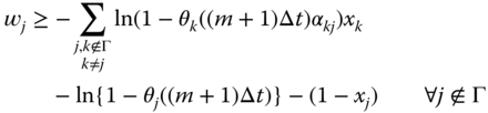
Equation (19.15) is necessary to ensure that EVSEs are kept connected to the network whenever their threat levels do not exceed the threshold value.
Isolating EVSEs may affect the power supply to EVs. Therefore, we should ensure that supply meets demand.
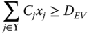
where ![]() is the capacity of
is the capacity of ![]() and
and ![]() is the forecast demand for the EV‐charging stations at
is the forecast demand for the EV‐charging stations at ![]() .
.
19.6 Propagation Impacts on Power System Operations
As discussed earlier, a cyberattack to PETS may further propagate to utility servers and from there, on to other power system modules such as the generator software or utility PMU networks. In this chapter, we also study propagation of cyberattacks in PMU networks for two reasons. First, since PMU networks are more protected and harder to attack, a cyberattacker, aiming for the PMU networks, may initiate the attack from PETS. More importantly, PETS components, similar to PMUs, will become connected through a communication network, which could expedite propagation of cyberattacks. Studying the propagation of cyberattacks in PMU networks sheds light on the future of the interconnected PETS and puts more emphasis on the necessity of response models against cyberattacks propagation in PETS.
19.6.1 Cyberattack Propagation in PMU Networks
PMUs measure the synchronized phasors of bus voltages and currents in real time for more accurate observability of the power grid (Dua et al., 2008). A PMU takes about 30 to 120 measurements per second and sends its measurements to a phasor data concentrator (PDC) through a wireless communication network based on the NASPInet architecture (Wang, 2013; NASPOnet, 2009). In the NASPInet architecture, PMUs are connected to an IP‐based communication network such as an Intranet. Although the communication network is a dedicated Intranet and is isolated from public networks, it is not immune to cyberattacks (Lin, 2012). A technical report from CISCO proposes that PMUs should send measurements using the IP multicast routing protocol (Cisco, 2012). In this communication protocol, a PMU is directly connected to a router and sends out data packets to pre‐configured destinations. The list of these predetermined destinations is a great target for cyberattackers to propagate the cyberattack to other PMUs. Furthermore, it has been reported that the communication network shows poor network security and insufficient software security (INL, 2010). Under these conditions, cyberattackers could gain access to the PMU communication network, inject false measurement data, and propagate their cyberattack to the other PMUs, jeopardize the observability of the power system, and put safe operations of the power grid at risk. The summary of notations used throughout the next section is given in Table 19.2.
19.6.2 Threat Level Estimation in PMU Networks
It is assumed that ![]() PMUs are detected to be compromised at time
PMUs are detected to be compromised at time ![]() . It takes time
. It takes time ![]() to disable the compromised PMUs from the communication network. Naturally, their measurements will no longer be used for the observability of the system. During time
to disable the compromised PMUs from the communication network. Naturally, their measurements will no longer be used for the observability of the system. During time ![]() , there is a chance that the attack could have been propagated to uncompromised PMUs and the detection software has not detected them yet. The reason is that the detection software cannot detect at 100% efficiency (INL, 2010). The cyberattack propagates to other PMUs through a path of interconnected routers in the communication network. If the cyberattack successfully breaks into all routers between the compromised and uncompromised PMUs, it is likely to contaminate the uncompromised PMUs as well. These newly compromised PMUs further contaminate other PMUs, and so forth. We represent by the probability,
, there is a chance that the attack could have been propagated to uncompromised PMUs and the detection software has not detected them yet. The reason is that the detection software cannot detect at 100% efficiency (INL, 2010). The cyberattack propagates to other PMUs through a path of interconnected routers in the communication network. If the cyberattack successfully breaks into all routers between the compromised and uncompromised PMUs, it is likely to contaminate the uncompromised PMUs as well. These newly compromised PMUs further contaminate other PMUs, and so forth. We represent by the probability, ![]() , the likelihood of a PMU being compromised (also called threat level) at time
, the likelihood of a PMU being compromised (also called threat level) at time ![]() . Notice that threat levels increase over time as long as the network still contains compromised PMUs. It takes a time period of
. Notice that threat levels increase over time as long as the network still contains compromised PMUs. It takes a time period of ![]() for the system operator to run the optimization model to obtain the optimal response and confirm that the alarm is not a false alarm. Thus, certain PMUs, determined by the optimization model, are disabled at time
for the system operator to run the optimization model to obtain the optimal response and confirm that the alarm is not a false alarm. Thus, certain PMUs, determined by the optimization model, are disabled at time ![]() . At time
. At time ![]() , equations (19.17) and (19.18) hold.
, equations (19.17) and (19.18) hold.
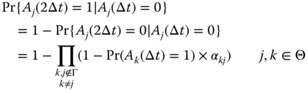
All detected compromised PMUs are disabled by time ![]() . However, it is likely that the attack could have been propagated to other PMUs but not detected yet. Therefore at time
. However, it is likely that the attack could have been propagated to other PMUs but not detected yet. Therefore at time ![]() , equations (19.19) and (19.20) hold.
, equations (19.19) and (19.20) hold.
where ![]() is the probability that the attack propagates from compromised
is the probability that the attack propagates from compromised ![]() to an uncompromised
to an uncompromised ![]() during the time
during the time ![]() , and it is given by equation (19.21).
, and it is given by equation (19.21).
In equation ( 19.21), ![]() is the probability that an attack propagates through a router,
is the probability that an attack propagates through a router, ![]() represents the probability that an attack propagates to another PMU and
represents the probability that an attack propagates to another PMU and ![]() , called nodal distance, is the minimum number of routers that connect
, called nodal distance, is the minimum number of routers that connect ![]() and
and ![]() on the communication network.
on the communication network.
Table 19.2 Summary of notations.
| Notation | Definition |
|
|
Set of buses |
|
|
Set of buses equipped with PMUs |
|
|
Set of PMUs detected as compromised |
|
|
Set of buses with conventional devices |
|
|
Set of branches with conventional devices |
|
|
Indices of buses |
|
|
Number of detected compromised PMUs |
|
|
Connectivity between buses |
|
|
Threshold threat level (between 0 and 1) of |
|
|
Nodal distance between |
|
|
Time that a propagation attempt takes |
|
|
Number of |
|
|
Binary decision variable which equals 1 if |
|
|
Observability number, number of times that bus |
|
|
Binary variable which equals 1 if the measurement from the conventional device at bus |
|
|
Binary variable which equals 1 if the measurement from the conventional device at transmission line |
|
|
random variable which equals 1 if |
|
|
The probability that |
|
|
The probability that an attack propagates through a router |
|
|
The probability that an attack propagates to a PMU through a router |
|
|
The threat level of |
As mentioned earlier, disabling the compromised PMUs takes time ![]() . Disabled PMUs would be enabled again if, during
. Disabled PMUs would be enabled again if, during ![]() , the system operator ensures that the alarm was false. If the alarm was true, the operator disables the PMUs as determined by the optimization model at
, the system operator ensures that the alarm was false. If the alarm was true, the operator disables the PMUs as determined by the optimization model at ![]() . Compromised PMUs would be disabled by time
. Compromised PMUs would be disabled by time ![]() . Therefore, the threat levels at time
. Therefore, the threat levels at time ![]() need to be calculated. Since the threat levels are calculated in an iterative process, we need to calculate the threat levels at time
need to be calculated. Since the threat levels are calculated in an iterative process, we need to calculate the threat levels at time ![]() ,
, ![]() ,
, ![]() ,
, ![]() . Equations (19.22) and (19.23) hold at time
. Equations (19.22) and (19.23) hold at time ![]() .
.

In equation ( 19.23), we have expressions for all terms except for ![]() , which can be obtained from equation (19.24).
, which can be obtained from equation (19.24).
We denote ![]() by
by ![]() . Therefore, we can rewrite equation ( 19.23) as equation (19.25) in terms of threat levels.
. Therefore, we can rewrite equation ( 19.23) as equation (19.25) in terms of threat levels.
Equation (19.26) holds when ![]() . Hence, we use equation ( 19.26) to estimate the threat levels for time
. Hence, we use equation ( 19.26) to estimate the threat levels for time ![]() .
.

19.6.3 Response Model in PMU Networks
The response to cyberattacks to a PMU network is modeled using mixed integer linear programming. In this optimization model, the objective function minimizes the maximum threat level of the PMUs that remain connected to the network at time ![]() . Time
. Time ![]() is one
is one ![]() after disabling the PMUs determined to be disabled by the proposed optimization model. We summarize the threat levels from time
after disabling the PMUs determined to be disabled by the proposed optimization model. We summarize the threat levels from time ![]() to
to ![]() in equations (19.27)–(19.33).
in equations (19.27)–(19.33).


The binary decision variable ![]() in equation ( 19.33) equals 0 if the
in equation ( 19.33) equals 0 if the ![]() is disconnected from the network. The system operator cannot control the threat levels from time
is disconnected from the network. The system operator cannot control the threat levels from time ![]() to
to ![]() . This is due to the network constraints such as control and communication delays in disconnecting PMUs. Disabling the selected PMUs occurs at time
. This is due to the network constraints such as control and communication delays in disconnecting PMUs. Disabling the selected PMUs occurs at time ![]() , which decreases the threat levels from time
, which decreases the threat levels from time ![]() . The response optimization model disables PMUs such that the maximum threat levels at time
. The response optimization model disables PMUs such that the maximum threat levels at time ![]() is minimized. Equation ( 19.33) is represented linearly in equation (19.34) to be solved more efficiently.
is minimized. Equation ( 19.33) is represented linearly in equation (19.34) to be solved more efficiently.

The following equality is used to obtain equation ( 19.34). Notice that the parameter ![]() is constant and
is constant and ![]() is a binary variable.
is a binary variable.
The objective function of the response model is to minimize of the maximum threat level of all connected PMUs at time ![]() .
.
![]() and therefore the objective function is not linear. We use its equivalent function, given in equation (19.37) and reformulate it linearly using equations (19.38)–(19.43).
and therefore the objective function is not linear. We use its equivalent function, given in equation (19.37) and reformulate it linearly using equations (19.38)–(19.43).
To find the linear equivalent of the objective function, we use equations ( 19.38)–( 19.43) to represent equation ( 19.37).
Subject to:
In the response model, we used equation ( 19.34) in equations (19.40)–(19.41) to obtain equivalent linear equations. Hence, equations ( 19.40)–( 19.41) can be represented as equations (19.44)–(19.45), respectively.

We add equation (19.46) to avoid disabling PMUs whose threat levels do not exceed the threshold value.
which can be represented by:
The right‐hand side can be reformulated as a linear equation as:

Using equation ( 19.34), equation (19.48) can be represented linearly as equation (19.49).

Disabling PMUs may affect the observability of the power system. Equation (19.50) provides the observability function introduced in [37].
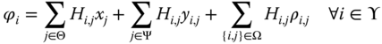
Where ![]() is the connectivity matrix.
is the connectivity matrix. ![]() determines the observability of the buses through PMUs still connected to the network;
determines the observability of the buses through PMUs still connected to the network; ![]() represents the observability of the buses through conventional devices installed at buses, and
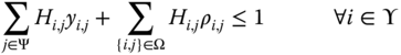
represents the observability of the buses through conventional devices installed at buses, and ![]() calculates the observability of the buses through conventional devices installed on transmission lines. Equation (19.51) ensures that there is at least one measurement to make each bus observable.
calculates the observability of the buses through conventional devices installed on transmission lines. Equation (19.51) ensures that there is at least one measurement to make each bus observable.
Conventional devices provides observability for a group of buses that are not directly measured by PMUs. In such cases, a system of equations needs to be solved in order to obtain the unknown state variables. Each conventional measurement needs to be assigned to one state variable, given in equations (19.52)–(19.53), to guarantee the solvability of the system of equations [37]. Equation ( 19.52) assigns one state variable to each conventional voltage measurement device, whereas equation ( 19.53) assigns one state variable to each conventional current measurement device. Equation (19.54) forces the measurements of conventional devices to observe more buses since measurements obtained by conventional devices are more reliable at the time of cyberattacks.
where the decision variable ![]() determines whether the state variable of bus
determines whether the state variable of bus ![]() is obtained by a conventional device at branch
is obtained by a conventional device at branch ![]() . The decision variables are binary and given in equation (19.55).
. The decision variables are binary and given in equation (19.55).
19.6.4 PMU Networks: Experimental Results
The performance of our response model is tested on the 6‐bus test system. We use the 6‐bus test system, introduced in [38], to explain the problem of study and our methodology. The 6‐bus test system, depicted in Figure 19.1, consists of six buses, eleven transmission lines, and three generators.

Figure 19.1 The 6‐bus test system
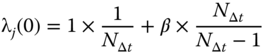
In our experiments, we assume that an attack to a PMU propagates through a router with probability ![]() , and it effectively compromises another PMU with probability
, and it effectively compromises another PMU with probability ![]() . For simplicity, we also assume that there is only one shortest path between PMUs. We set
. For simplicity, we also assume that there is only one shortest path between PMUs. We set ![]() . We set
. We set ![]() to 0.1 seconds,
to 0.1 seconds, ![]() (s), and the threshold values to 0.005,
(s), and the threshold values to 0.005, ![]() .
.
To ensure full and redundant observability, it is assumed that PMUs are installed at buses 1, 2, 3, 4, and 6. The communication network, shown in Figure 19.1, consists of interconnected routers to send PMU measurements to PDCs. PMUs' nodal distances are given in Table 19.3.
Table 19.3 6‐bus test system – Nodal distances.
| Bus | 1 | 2 | 3 | 4 | 6 |
| 1 | 0 | 2 | 3 | 1 | 2 |
| 2 | 2 | 0 | 3 | 3 | 2 |
| 3 | 3 | 3 | 0 | 1 | 2 |
| 4 | 1 | 3 | 1 | 0 | 3 |
| 6 | 2 | 2 | 2 | 3 | 0 |
For this case study, we assume that at time ![]() the system operator is informed that
the system operator is informed that ![]() and
and ![]() have been attacked by a cyber‐intruder. In Figure 19.2, we show the threat levels of the three uncompromised PMUs over time when the system operator does not disable the compromised PMUs from the network. Notice that the threat levels increase nonlinearly until all PMUs become compromised with probability 1.
have been attacked by a cyber‐intruder. In Figure 19.2, we show the threat levels of the three uncompromised PMUs over time when the system operator does not disable the compromised PMUs from the network. Notice that the threat levels increase nonlinearly until all PMUs become compromised with probability 1. ![]() is more at risk because it is closer to the compromised PMUs. The nodal distance from
is more at risk because it is closer to the compromised PMUs. The nodal distance from ![]() to
to ![]() is 1 while to
is 1 while to ![]() is 3. Figure 19.3 illustrates the effect of the value of
is 3. Figure 19.3 illustrates the effect of the value of ![]() on the threat level of
on the threat level of ![]() .
.
Table 19.4 Candidate responses for the 6‐bus test system.
| PMU | Candidate Response | |||||||
| Status | 1 | 2 | 3 | 4 | 5 | 6 | 7 | 8 |
|
|
1 | 1 | 1 | 1 | 0 | 0 | 0 | 0 |
|
|
1 | 0 | 0 | 1 | 1 | 0 | 1 | 0 |
|
|
1 | 1 | 0 | 0 | 1 | 1 | 0 | 0 |
| Threat Levels | ||||||||
|
|
0.00013 | 0.00013 | 0.00013 | 0.00013 | 0 | 0 | 0 | 0 |
|
|
0.00500 | 0 | 0 | 0.00500 | 0.00500 | 0 | 0.00500 | 0 |
|
|
0.00025 | 0.00025 | 0 | 0 | 0.00025 | 0.00025 | 0 | 0 |
|
Max(
|
0.00500 | 0.00025 | 0.00013 | 0.00500 | 0.00500 | 0.00025 | 0.00500 | 0 |
| Observaiblity | Yes | Yes | Yes | Yes | Yes | No | No | No |
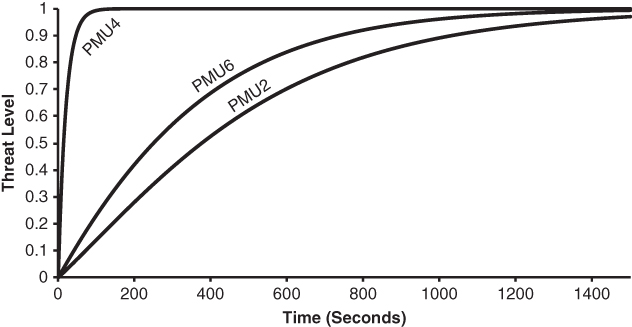
Figure 19.2 Threat levels in case of no response action

Figure 19.3
Effect of  on threat level of
To avoid propagation, the system operator should disable the compromised ![]() and
and ![]() and other PMUs that may be compromised because of the propagation. There are eight possible choices, which are shown in Table 19.4. The smallest threat levels can be obtained when all PMUs are disabled. However, this solution is not feasible since the power system would no longer be observable. The second candidate is to disable
and other PMUs that may be compromised because of the propagation. There are eight possible choices, which are shown in Table 19.4. The smallest threat levels can be obtained when all PMUs are disabled. However, this solution is not feasible since the power system would no longer be observable. The second candidate is to disable ![]() and
and ![]() , but the threat level of
, but the threat level of ![]() is less than the threshold value,
is less than the threshold value, ![]() , and therefore it should remain connected to the network. The third candidate is to disable
, and therefore it should remain connected to the network. The third candidate is to disable ![]() . This action keeps the power network observable and minimizes the maximum threat level of all connected PMUs. In Table 19.5, we give the optimal solution, observability number of the buses obtained from equation ( 19.50) and the threat level of each connected PMU right after disabling
. This action keeps the power network observable and minimizes the maximum threat level of all connected PMUs. In Table 19.5, we give the optimal solution, observability number of the buses obtained from equation ( 19.50) and the threat level of each connected PMU right after disabling ![]() .
.
Table 19.5 6‐bus system – Optimal response
| PMU |
|
Observability number |
Threat level |
| 1 | 0 | 1 | 0 |
| 2 | 1 | 2 | 0.00013 |
| 3 | 0 | 2 | 0 |
| 4 | 0 | 1 | 0 |
| 5 | NA | 2 | NA |
| 6 | 1 | 2 | 0.00025 |
In Figure 19.4, the maximum threat levels of the connected PMUs are compared for two potential responses, 1) disconnecting only the compromised PMUs, and 2) disconnecting ![]() in addition to the compromised PMUs (optimal response). Although the threat levels still increase after the response action, the reduction in threat levels after the optimal response is considerable.
in addition to the compromised PMUs (optimal response). Although the threat levels still increase after the response action, the reduction in threat levels after the optimal response is considerable.

Figure 19.4 Comparison of two potential responses
To study how the optimization time affects the threat levels, we consider that the optimal results will be obtained in 0.1, 2, and 5 seconds. The optimal decision, in all three cases, is to disconnect ![]() . The results are compared in Figure 19.5, which suggests that a shorter processing time is desired.
. The results are compared in Figure 19.5, which suggests that a shorter processing time is desired.

Figure 19.5
Threat level of  for different computational times
19.7 Conclusion and Open Issues
This chapter introduced the security vulnerabilities of smart cities from the smart grid and smart transportation perspective. We focused on EVs and PMUs, as they present point of access for cyber‐ threats; however, our approach can be easily generalized to any smart city asset. We introduced threat level computation and its corresponding response model.
Future work needs to investigate more on the response models and their implications on the service and observability side. Traditional response models isolate equipment in order to isolate attacks. Yet, in systems with inadequate redundancy this may cause disruption of service. One important open issue is to investigate the trade‐off between redundancy investment and protection provided.
References
- 1 Lloyds (2015) Center for Risk Studies, University of Cambridge, “Lloyd's Emerging Risk Report, Business Blackout” [Online] www.lloyds.com
- 2 Fireeye (2017) Fireeye Inc. Cyber Threat Map. https://www.fireeye.com/cyber‐map/threat‐map.html
- 3 C. Cerrudu (2015) “An Emerging US (and World) Threat: Cities Wide Open to Cyber Attacks.” [Online] https://securingsmartcities.org/wp‐content/uploads/2015/05/CitiesWideOpenToCyberAttacks.pdf
- 4 DoE (2009) U.S. Department of Energy Office of Electricity Delivery and Energy Reliability, “Study of Security Attributes of Smart Grid Systems – Current Cyber Security Issues”. [Online] http://www.inl.gov/scada/publications/d/securing_the_smart_grid_current _issues.pdf.
- 5 DoE (2012) U.S. Department of Energy Office, Electricity Subsector Cybersecurity Risk Management Process. [Online] http://energy.gov/oe/downloads/cybersecurity‐risk‐management‐process‐rmp‐guideline‐final‐may‐2012.
- 6 C. Carryl, M. Ilyas, I. Mahgoub, M. Rathod, (2013) “The PEV security challenges to the smart grid: Analysis of threats and mitigation strategies,” International Conference on Connected Vehicles and Expo (ICCVE), pp. 300–305, 2‐6.
- 7 S. Mousavian, J. Valenzuela, J. Wang, (2014) “A Probabilistic Risk Mitigation Model for Cyber Attacks to PMU Networks,” in IEEE Transactions on Power Systems, vol. 30, no. 1, pp. 156–165.
- 8 S. Mousavian, M. Erol‐Kantarci, T. Ortmeyer, (2015) “Cyber Attack Protection for a Resilient Electric Vehicle Infrastructure,” IEEE Globecom‐Workshop on Smart Grid Resilience, San Diego, CA, pp. 1–6.
- 9 Y. Li, R. Wang, P. Wang, D. Niyato, W. Saad, Z. Han (2012) “Resilient PHEV charging policies under price information attacks,” IEEE Third International Conference on Smart Grid Communications (SmartGridComm), pp. 389–394, 5‐8.
- 10 S. A. Khayam, H. Radha (2004) “Analyzing the spread of active worms over VANET,” Proceedings of the 1st ACM international workshop on Vehicular ad hoc networks, pp. 86–87.
- 11 J. W. Mickens, B. D. Noble (2005) “Modeling epidemic spreading in mobile environments,” Proceedings of the 4th ACM workshop on Wireless security, pp. 77–86.
- 12 R. Northfield (2016) “Greening the smart city,” IEEE Engineering & Technology, vol. 11, no. 5, pp. 38–41, June 2016.
- 13 R. Khatoun and S. Zeadally (2017) “Cybersecurity and Privacy Solutions in Smart Cities,” in IEEE Communications Magazine, vol. 55, no. 3, pp. 51–59.
- 14 K. Zhang, J. Ni, K. Yang, X. Liang, J. Ren and X. S. Shen (2017) “Security and Privacy in Smart City Applications: Challenges and Solutions,” in IEEE Communications Magazine, vol. 55, no. 1, pp. 122–129.
- 15 J.A.P. Lopes, F. J. Soares, P. M. R. Almeida (2011) “Integration of Electric Vehicles in the Electric Power System,” Proceedings of the IEEE, Vol. 99, No. 1, pp. 168–183.
- 16 W.C. Su, H. Rahimi‐Eichi, W.T. Zeng, M.Y. Chow (2012) “A survey on the electrification of transportation in a smart grid environment,” IEEE Transactions on Industrial Informatics, vol. 8, pp. 1–10.
- 17 H. T. Mouftah, M. Erol‐Kantarci (2012) “Smart Grid Communications: Opportunities and Challenges,” Handbook of Green Information and Communication Systems, Eds. M. S. Obaidat, A. Anpalagan and I. Woungang, Elsevier.
- 18 D. Niyato, N. Kayastha, E. Hossain, and Z. Han (2014) “Smart grid sensor data collection, communication, and networking: A tutorial,” Wireless Communications and Mobile Computing (Wiley), vol. 14, no. 11, pp. 1055–1087.
- 19 M. Simpson, M. Jun, M. Kuss, T. Markel (2012) “Demonstrating PLC over J1772 During PEV Charging for Application at Military Microgrids.” [Online] http://mydocs.epri.com/docs/PublicMeetingMaterials/0712/D2‐4.pdf.
- 20 K. Mets, T. Verschueren, W. Haerick, C. Develder, F. De Turck (2010) “Optimizing smart energy control strategies for plug‐in hybrid electric vehicle charging,” IEEE/IFIP Network Operations and Management Symposium Workshops, pp. 293–299.
- 21 K. Clement, E. Haesen, J. Driesen (2009) “Coordinated charging of multiple plug‐in hybrid electric vehicles in residential distribution grids,” IEEE Power Systems Conference and Exposition, pp. 1–7.
- 22 E. Sortomme, M.M. Hindi, S. D. J. MacPherson, S. S. Venkata (2011) “Coordinated Charging of Plug‐In Hybrid Electric Vehicles to Minimize Distribution System Losses,” IEEE Transactions on Smart Grid, vol. 2, no. 1, pp. 198–205.
- 23 M. Erol‐Kantarci, J. H. Sarker, H. T. Mouftah (2011) “Communication‐based Plug‐in Hybrid Electrical Vehicle Load Management in the Smart Grid,” IEEE Symposium on Computers and Communications, pp. 404–409.
- 24 S.M. Amin, B.F. Wollenberg (2005) “Toward a smart grid: power delivery for the 21st century,” IEEE Power and Energy Magazine, vol. 3, no. 5, pp. 34–41.
- 25 X. Fang, S. Misra, G. Xue, D. Yang (2012) “Smart Grid ‐ The New and Improved Power Grid: A Survey,” IEEE Communications Surveys & Tutorials, vol. 14, no. 4, pp. 944–980.
- 26 Y. Yan, Y. Qian, H. Sharif, and D. Tipper (2012) “A Survey on Cyber Security for Smart Grid Communications,” IEEE Communications Surveys and Tutorials, Vol. 14, Issue 4, pp. 998–1010.
- 27 S. M. Amin and A. M. Giacomoni (2012) “Smart Grid‐ Safe, Secure, Self‐Healing: Challenges and Opportunities in Power System Security, Resiliency, and Privacy,” IEEE Power & Energy Magazine, pp. 33–40.
- 28 A. C‐F. Chan and J. Zhou (2013) “On smart grid cybersecurity standardization: Issues of designing with NISTIR 7628,” IEEE Communication Magazine, vol. 51, no. 1, pp. 58–65.
- 29 A. C.‐F. Chan, J. Zhou (2014) “Cyber‐physical device authentication for smart grid electric vehicle ecosystem,” IEEE Journal on Selected Areas in Communications, Vol. 32, 1509–1517.
- 30 D. Dua, S. Dambhare, R. K. Gajbhiye, and S. A. Soman (2008) “Optimal multistage scheduling of PMU placement: An ILP approach,” IEEE Transactions on Power Delivery, vol. 23, pp. 1812–1820.
- 31 W. Wang and Z. Lu (2013) “Cyber security in the smart grid: Survey and challenges,” Computer Networks.
- 32 NASPInet (2009) Data bus technical specifications for north american syncro‐phasor initiative network (NASPInet). North American Syncro‐Phasor Initiative Network. [Online]. Available: https://www.naspi.org/File.aspx?fileID=587
- 33 H. Lin, Y. Deng, S. Shukla, J. Thorp, and L. Mili (2012) “Cyber security impacts on all‐PMU state estimator a case study on co‐simulation platform GECO,” in IEEE Third International Conference on Smart Grid Communications (SmartGridComm), pp. 587–592.
- 34 Cisco (2012) PMU networking with IP multicast. CISCO Public. [Online]. Available: http://www.cisco.com/
- 35 INL (2010) “NSTB assessments summary report: Common industrial control system cyber security weaknesses,” Idaho National Laboratory (INL), Tech. Rep.
- 36 C. Shuguang, H. Zhu, S. Kar, T. T. Kim, H. V. Poor, and A. Tajer (2012) “Coordinated data‐injection attack and detection in the smart grid: A detailed look at enriching detection solutions,” IEEE Signal Processing Magazine, vol. 29, pp. 106–115.
- 37 S. Azizi, B. G. Gharehpetian, G. Hug‐Glanzmann, and A. Dobakhshari (2012) “Optimal integration of phasor measurement units in power systems considering conventional measurements,” IEEE Transactions on Smart Grid, vol. 4, pp. 1113–1121.
- 38 A. J. Wood and B. F. Wollenberg (1996) Power Generation, Operation and Control. John Wiley & Sons.
- 39 IEEE Test System (1979) Subcommittee, “IEEE reliability test system,” IEEE Transactions on Power Apparatus and Systems, vol. 98, pp. 2047–2054.