
10
A Prediction Module for Smart City IoT Platforms
Sema F. Oktug Yusuf Yaslan and Halil Gulacar
Computer Engineering Department, Istanbul Technical University, Istanbul, Turkey
10.1 Introduction
Today, nearly all types of sensors have a wireless network connection with data sending and receiving capacity, which brings the device connectivity, namely Internet of things (IoT) technologies, to our daily life. IoT is a paradigm that enables communication between objects (anything and anyone) at any time and any place. IoT is widely used in different application areas such as home automation, health, traffic, manufacturing, etc. With the advance of the IoT technologies, increasing amount of data became available from sensors distributed around the cities. Big data technologies and machine learning algorithms enable services and solutions to citizens and decision makers by using these urban data.
The rapid urbanization in the last century required the decision makers to increase the citizens' quality of life and make appropriate investments in infrastructure. Nowadays, utilization of energy resources, smart traffic management, air pollution, waste management, and other urban‐related issues are critical. The prediction systems are required in these fields in order to improve the quality of services and solutions. For instance, a smart traffic application that has prediction capability can help dwellers to forecast the traffic jams and arrange their routes before going out. Similarly, prediction of the solid waste generation also helps to plan and design waste management systems. Prediction of air pollutants such as carbon monoxide (CO), ozone (O3), sulphur dioxide (SO2) and nitrogen dioxide (NO2) in the air is crucial for public health, and recently urban air pollution is becoming a more serious problem (Mehta et. al., 2016). Therefore, air quality systems should include quality predictions for government authorities to take cautions against pollution. Another important aspect of smart cities is an efficient energy management system and smart grid concept where more renewable energy resources are utilized. In order to have a better energy management, it is crucial to effectively predict the renewable power generation from solar and wind resources (Wang et. al., 2015). Besides, it is also important to forecast the electric load demands for energy management. Like in power grid systems, in all of the demand‐and‐supply‐based management systems and applications having similar structure, predicting demand is very important. If you predict the demand of the next day and see that it is more than the supply available and if you could not increase the supply, you should find ways to reduce demand in order not to cause shortages. In addition to the aforementioned applications, another problem for drivers in crowded cities is to find parking places in the city. Hence, parking availability prediction becomes crucial (Vlahogianni et. al., 2015). Most of these examples use predictions in practice, and the number of such examples that are showing the importance of prediction could be increased. Hence, we could say that the prediction‐based services/solutions, especially the ones related to the cities, are very valuable for the citizens.
Nowadays, most of these services are provided by IoT platforms that are developed by using different technologies for different purposes. Many IoT platforms have been previously developed, and a comprehensive comparison of most of the IoT platforms are given in Köhler, Wörner, and Wortmann (2014). However, that work is not dedicated to smart city IoT platforms, and as the technology evolves rapidly, the number of platforms and their capabilities are changing day by day. Hence, the need for systematic evaluation of the capabilities of smart city IoT platforms is increasing. On the other hand, cloud computing environments enable scalable smart city platforms that combine multiple stakeholders' services. Cloud platforms also support rapid application development by serving programming tools, environments, and data storage area. Hence, cloud support to any IoT platform recently became inevitable.
In this work, we first introduce recently developed IoT platforms for smart city applications. These platforms could be listed as ARMmbed (Mbed, 2016), Cumulocity (Cumulocity, 2016), DeviceHive (DeviceHive, 2015), Digi (Digi, 2016), Digital Service Cloud (Digital Service Cloud, 2015), FiWare (FIWARE, 2011), GSN (GSN, 2016), IoTgo (IoTgo, 2014), Kaa (Kaa, 2014), Nimbits (Nimbits, n.d.), RealTime.io (RealTime.io, 2016), SensorCloud (SensorCloud, 2016), SiteWhere (SiteWhere, 2009), TempoIQ (TempoIQ, 2016), Thinger.io (Thinger.io, 2016), Thingsquare (Thingsquare, n.d.), ThingWorx (ThingWorx, 2016), Xievly (Xively, 2016), Vital (VITAL, 2016), chronologically. We compare them with respect to the cloud systems employed, communication protocols, authentication methods, database types, and prediction capabilities.
Next, we focus to the prediction module developed for the Vital platform by
- providing information about the prediction methods employed;
- showing the results obtained for the traffic speed sensors of the Istanbul Metropolitan Municipality, and evaluating the results by using the root mean squared error measure; and
- explaining the integration of the prediction module to the Vital platform.
The acronyms used throughout the chapter are listed below:
- IoT: Internet of things
- ARM: Acorn‐advanced RISC machine
- OS: operating system
- Bluetooth LE: Bluetooth low energy
- Wi‐Fi: wireless fidelity
- CoAP: constrained application protocol
- MQTT: message queue telemetry transport
- HTTP: yyper‐text transfer protocol
- REST: representational state transfer
- OWASP: open web application security project
- HDFS: hadoop‐distributed file system
- CoAP: constrained application protocol
- XMPP: extensible messaging and presence protocol
- API: application programming interface
- PaaS: platform as a service
The chapter is organized as follows. In Section , we give details about the IoT platforms for smart cities and compare them in a table. Next, Section introduces the developed prediction module and the VITAL IoT platform. Section details the use case application developed for speed prediction and presents the experimental results obtained. The chapter is concluded by summarizing the results obtained and giving future directions.
10.2 IoT Platforms for Smart Cities
In this section, we will cover 18 IoT platforms introduced for smart cities in terms of their cloud support, communication protocols, authentication mechanisms, databases, and prediction capabilities. First, we introduce the IoT platforms by giving brief information about their capabilities. Detailed comparison of these platforms is given in Table 10.1.
Table 10.1 Comparisons of IoT‐Based Smart City Platforms.
| Platforms | Cloud | Communication protocols | Authentication | Database | Prediction opportunity |
| ARMmbed | ARMmbed cloud | CoAP; MQTT; HTTP/REST | ‐ | ‐ | ‐ |
| Cumulocity | Cumulocity cloud | HTTP/REST | OAuth2 | ‐ | Cumulocity analytics |
| DeviceHive | On‐premises; cloud; hosted; hybrid | MQTT; HTTP/REST | OAuth2; HTTP basic authentication | MongoDB | ElasticSearch, Apache Spark, Cassandra, and Kafka |
| Digi | Digi Cloud | HTTP/REST | HTTP basic authentication | ‐ | ‐ |
| Digital Service Cloud | Microsoft Azure | HTTP/REST | OWASP | MongoDB; SQL Server | Azure machine learning |
| FiWare | FiWare cloud | MQTT; HTTP/REST | OAuth2 | Hadoop; MongoDB | TrafficHeat (In FiWare Hackathon big data) |
| GSN | On‐premises | HTTP/REST, SOAP; MQTT; CoAP | HTTP basic authentication | MySQL | Weka |
| IoTgo | On‐premises; cloud; Hosted; hybrid | HTTP/REST; WebSocket | HTTP basic authentication | MongoDB | ‐ |
| Kaa | On‐premises; cloud; hosted; hybrid | MQTT; HTTP/REST; CoAP; XMPP | OAuth | Cassandra; MongoDB | Apache Spark |
| Nimbits | On‐premises; cloud; hosted | MQTT; XMPP; HTTP/REST | HTTP basic authentication | MySQL | ‐ |
| RealTime.io | ioBridge cloud | UDP‐based ioDP; HTTP/REST | HTTP basic authentication | ‐ | ‐ |
| SensorCloud | SensorCloud; Amazon Web Services | HTTP/REST | API key; HTTP basic authentication | SQL Azure | MathEngine; IPython and SciPy |
| SiteWhere | On‐premises; cloud; hosted; hybrid | MQTT; AMQP; Stomp; HTTP/REST | HTTP basic authentication | MongoDB; Apache HBase; InfluxDB | ‐ |
| TempoIQ | CODA Cloud | MQTT; HTTP/REST | ‐ | DataIQ | Analytic Composer |
| Thinger.io | Thinger Cloud | MQTT; HTTP/REST | OAuht2 | MongoDB | ‐ |
| ThingSquare | Thingsquare Cloud | HTTP/REST | HTTP basic authentication | ‐ | ‐ |
| ThingWorx | On‐premises; hosted; hybrid; ThingWorx cloud; Amazon Web Services; Microsoft Azure | CoAP; WebSockets; MQTT; HTTP/REST | HTTP basic authentication | Neo4j; Apache Casandra | ThingWorx Analytics |
| VITAL | On‐premises; cloud; hosted | HTTP /REST | HTTP basic authentication | MongoDB | Weka |
| Xively | Xively cloud | MQTT; HTTP/REST; WebSockets | OAuth2; HTTP basic authentication | Blueprint | ‐ |
10.2.1 ARM Mbed
Mbed (Mbed, 2016) IoT platform and operating system (OS) was released by ARM and licensed under Apache 2.0 in 2009. ARM is the company that produces microprocessors for mobile, IoT, wearable systems, automotive, health care, and other markets. Mbed OS is designed for IoT devices and includes the features necessary to develop a connected product based on ARM Cortex‐M microcontroller. Mbed OS is the core of the system and supports sensors and actuators and different communication technologies such as Wi‐Fi and Bluetooth LE. It also has a web‐based development environment. Mbed has its own cloud, named ARM Mbed Cloud. The source code written through web browsers is compiled in the cloud environment. Communication is provided by using CoAP, MQTT, and HTTP/RESTful protocols.
10.2.2 Cumulocity
The term “Cumulocity” is a compound of “Cumulus” (a type of cloud ) and “velocity.” It is Nokia's IoT spin‐off, founded in 2010 in Silicon Valley, California (Cumulocity 2016). Cumulocity GmbH continues development in Düsseldorf, Germany, with the support of Nokia Siemens Networks.
Cumulocity is an application‐centric IoT platform whose functionality is available for public via open APIs. Cumulocity has its own cloud system, and sensor nodes are clients that connect to this system through RESTful, HTTPS, and API. Data collection from devices and their remote management is done through the Cloud Fieldbus application. HTTP(S)/RESTful is the only supported communication protocol in Cumulocity (Derhamy et. al., 2001). It implements OAuth2 protocol for authentication. There is no information about the database system used. On the other hand, it has a system for real‐time data analytics.
10.2.3 DeviceHive
DeviceHive (DeviceHive, 2015) is an open‐source IoT data platform, which was introduced by an IoT research and development company, DataArt, in 2012. It supports the AllJoyn system, which allows devices to communicate with other devices around them. AllJoyn provides cloud connectivity for AllJoyn‐supported devices, and it can be used for as a bridge to connect with third‐party protocols.
DeviceHive is compatible with on‐premise, cloud, hosted, and hybrid systems. It works in public and private clouds: Microsoft Azure, Amazon Web Services, Apache Mesos, and OpenStack. It uses MQTT and HTTP/RESTful protocols for communication. DeviceHive has two authentication protocols: OAuth2 and HTTP basic authentication. It stores data in MongoDB and has support to many data analytics and big data tools such as ElasticSearch, Apache Spark, Cassandra, and Kafka. It supports real‐time and batch processing data analytic solutions.
10.2.4 Digi
Digi Inc. (Digi, 2016), which was founded in 1985, focused on PC boards in the first years. Then the company shifted toward M2M solutions such as satellite communication devices, integrated circuits, and gateways. Digi has started to proceed on its business with Etherios Inc., founded in 2008, and focused on the cloud sector since 2012. Respectively, the iDigi Energy and iDigi Tank platforms were developed for creating smart energy networks and monitoring tank storages. After adding the visualization tools of Thingworx and the cloud capabilities of Etherios, Digi became an advanced IoT platform (Köhler, Wörner, and Wortmann, 2014).
Digi has its own cloud, named Digi Cloud, for device integration and monitoring. It uses the HTTP/RESTful communication protocol and implements HTTP basic authentication protocol. On the other hand, there isn't any information about Digi's database system and data analytic services.
10.2.5 Digital Service Cloud
Digital Service Cloud Open IoT Platform (Digital Service Cloud, 2015) was launched by iYogi, New Delhi, in May 2015. It is built on Microsoft Azure and uses various Azure modules such as Service Bus, Event Hub, DocumentDB, and Machine Learning, for data analytics operations. Digital Service Cloud has more than 12 million connected devices, and it has the highest number of devices among digital service management platforms.
The infrastructure has the HTTP/RESTful communication protocol and OWASP for authentication service. Digital Service Cloud stores collected data in MongoDB and user data in Microsoft SQL Server.
10.2.6 FiWare
FiWare (FIWARE, 2011) is a middleware IoT platform developed by the FiWare community, which is an independent open community that aims to develop smart applications for various areas by constructing sustainable, open, and application‐driven middleware platform standards. It was supported by the European Union Future Internet Public‐Private Partnership (FI‐PPP) project's Framework Programme 7 (FP7) between 2011 and 2014 (COMM 2016). FiWare has its own cloud infrastructure, named FiWare Cloud, which is based on OpenStack. It uses MQTT and HTTP(S)/RESTful protocols for communication and the OAuth2 protocol for authentication. FiWare uses an HDFS‐based system for data storage and has a module named Cosmos for big data analysis. The TrafficHeat project used this module for traffic predictions in FiWare Big Data Hackathon (Santander‐Fiware, 2016).
10.2.7 Global Sensor Networks (GSN)
The Global Sensor Network (GSN, 2016) project is one of the initial projects that have been started in 2004 by Distributed Information Systems Laboratory LSIR at École Polytechnique Fédérale de Lausanne. It's an open‐source platform and is written in the Java programming language (Petrolo, Loscri, and Mitton, 2015). The main aim was to develop a middleware platform for sensor data integration and query processing. Later GSN is supported by other projects and institutions such as the OpenIoT project, the HYDROSYS project, and others. As it is one of the premise projects, it doesn't have any special cloud support and runs the on‐premise principle. While its first version uses HTTP/SOAP and RESTful communication protocols, MQTT and CoAP communication protocols were added in the second version. GSN implements HTTP basic authentication for authentication of users and uses a MySQL database for data storage. Although GSN has a Weka library that enables data analysis and mining operations, no application that predicts sensor observations by using this library was identified.
10.2.8 IoTgo
IoTgo (IoTgo, 2014) is an open‐source IoT platform founded by ITEAD Intelligent Systems Co. Ltd, which is headquartered in Shenzhen, China.
IoTgo is compatible with on‐premise, cloud, hosted, and hybrid systems. WebSocket and HTTP/RESTful are two communication protocols supported by IoTgo. IoTgo implements HTTP basic authentication method for authentication, and MongoDB is used for data storage. No information about data analytics has been found.
10.2.9 Kaa
Kaa (Kaa, 2014) is a middleware open‐source IoT platform that aims to collect information from various sources, and it is licensed under Apache 2.0. Since 2014, the Kaa project is an enterprise of CyberVision, a software company. Kaa has on‐premise, hosted, hybrid, and cloud deployments. It supports MQTT, HTTP(S)/RESTful, CoAP, and XMPP communication protocols and implements the OAuth authentication protocol. MongoDB and Cassandra databases are used for data storage. Collected data could be analyzed employing the Apache Spark extension of the platform. The Kaa project has endpoint SDKs for Java, C, C++, and Objective‐C.
10.2.10 Nimbits
Nimbits (Nimbits, n.d.) is an open‐source PaaS for IoT licensed under Apache 2.0. The Nimbits platform is compatible with Raspberry Pi, J2EE Web Application Servers, Amazon EC2, and the Google App Engine. It supports MQTT, XMPP, and HTTP/RESTful communication protocols and provides authentication by implementing HTTP basic authentication protocol. MySQL database is used to store the data. It provides Java libraries and SDK for development (Mazhelis and Tyrvainen, 2014). There is no information about data analytics and prediction systems in Nimbits.
10.2.11 RealTime.io
RealTime.io (RealTime.io, 2016) is a PaaS of ioBridge for IoT systems. The purpose of ioBridge RealTime.io is easy and cheap connection of products to the Internet and building a bridge between embedded systems and user applications.
RealTime.io has its own cloud system for storage and management. It uses UDP‐based ioDP (Mazhelis and Tyrvainen, 2014) and HTTP/RESTful protocol for communication and HTTP basic authentication for user and device authentication. There is no information about the database system employed and the data analytic tools of RealTime.io.
10.2.12 SensorCloud
SensorCloud (SensorCloud, 2016) is an IoT platform of US‐based LORD MicroStrain corporation. It was introduced by MicroStrain, founded in 1987. In the first years, the company focused on sensors used in biomedical research. MicroStrain released their first inertial product, the 3DM, in 1999. While it was initially thought of as a biomedical product, it was later made compatible with navigation systems, civil engineering projects, and industrial equipment monitoring. In 2001, MicroStrain released the first wireless sensor of the company. Owing to such a background, the company launched SensorCloud that enables to store, fast monitor, and analyze data in 2011. One year later, MicroStrain was acquired by LORD Corporation.
Sensor Cloud provides a cloud platform hosted by Amazon Web Services (AWS). It communicates via the HTTP/RESTful protocol and authenticates users via custom API key and HTTP basic authentication. It stores data in SQL Azure database. SensorCloud provides support to Python, Java, C#, and C++ (Mazhelis and Tyrvainen, 2014). It has also MathEngine, IPython, and Scipy support for data analysis and machine learning operations.
10.2.13 SiteWhere
SiteWhere (SiteWhere, 2009) is an IoT platform launched by SiteWhere LLC in 2009. The platform was initially aimed to be a telecommunications‐processing platform. Then real‐time location data has been integrated. And finally it became a more generalized IoT platform, and it is open‐sourced since June 2013.
SiteWhere is compatible with on‐premise, cloud, hosted, and hybrid systems. It communicates via the MQTT, AMQP, Stomp, and HTTP/RESTful protocols and implements HTTP basic authentication protocol. MongoDB, Apache HBase, and InfluxDB technologies are used for data storage. There isn't any information about predictive analytics usage by the SiteWhere platform.
10.2.14 TempoIQ
TempoIQ (TempoIQ, 2016), is an IoT platform developed with the purpose of providing fast, flexible, and agile device data collection, storage, and monitoring. TempoIQ uses the CODA cloud system for monitoring and controlling devices and data. Its communication protocols are MQTT and HTTP/RESTful. It provides support for C, Java, Python, Ruby and .NET (Mazhelis and Tyrvainen, 2014). TempoIQ stores data in the DataIQ module and has the Analytic Composer for data analysis in the AnalyticIQ module.
10.2.15 Thinger.io
Thinger.io (Thinger.io, 2016) is an IoT platform that has its own cloud infrastructure to connect and manage devices. It uses MQTT and HTTP/RESTful communication protocols. Users/customers can integrate it to their business logic by using REST API. Thinger.io authenticates users and devices by implementing the OAuth2 protocol, and collected data are stored in MongoDB. No information about prediction of device data has been found.
10.2.16 Thingsquare
The development of the Contiki Operating System, which is compatible with low‐power and less memory and suitable for connected devices, led to the foundation of ThingSquare (Thingsquare n.d.). Contiki and its commercial type ThingSquare Mist are released under the BSD license and open source (Köhler, Wörner, and Wortmann, 2014). ThingSquare focuses on mostly the automation, controlling, and monitoring of things via the Internet than integrating applications and analyzing collected data (Derhamy et. al., 2001). ThingSquare has its own cloud for deployment. It uses the HTTP/RESTful communication protocol and HTTP basic authentication method for authentication. ThingSquare has an IDE named “ThingSquare Code,” which enables development of applications for ThingSquare Mist. There isn't any information about its database and data analytics capabilities.
10.2.17 ThingWorx
ThingWorx (ThingWorx, 2016) is an IoT platform that reduces complexity for non‐technical people (Köhler, Wörner, and Wortmann, 2014). It focuses on integration, transformation, and presentation of collected data instead of communication between nodes and collection of data. Four main blocks of ThingWorx were built in 2011. The first block, SQUEAL, enables to search data and devices. The second one, Mashup Builder block, enables application development by “drag and drop.” The third block, Composer, was developed for composition of different data visualizations, storages. and business logics. Finally, the social networks block is used for crowdsourcing (Köhler, Wörner, and Wortmann, 2014). ThingWorx enables on‐premise, hosted, and hybrid deployments (Mazhelis and Tyrvainen, 2014). Besides, it is also compatible with third‐party clouds such as Amazon Web Services and Microsoft Azure. Thingworx uses CoAP, WebSockets, MQTT, and HTTP/RESTful communication protocols (Derhamy et. al., 2001) and implements HTTP basic authentication as authentication protocol. It stores model data in Apache Casandra, supports Neo4j graph database, and has a module named ThingWorx Analytics for data analytics.
10.2.18 VITAL
The VITAL (Virtualized programmable InTerfAces for smart, secure, and cost‐effective IoT depLoyments in smart cities; VITAL, 2016) platform aims to integrate inter‐connected objects (ICOs) among multiple IoT platforms. The detailed description of the platform will be given in the following sections.
10.2.19 Xively
Xively (Xively, 2016) is another a PaaS platform that enables real‐time communication, device monitoring, and data storage and distribution (Mazhelis and Tyrvainen, 2014). It was initially developed in 2007 to connect things to things and was named Pachube. In 2011 it was widely used in Japan to monitor radioactive fallout across the country after the nuclear accident in Fukushima. Then in the same year it was acquired by LogMeln and renamed Cosm. Later on in 2013, it was renamed Xively (Köhler, Wörner and Wortmann, 2014). Xively supports MQTT, HTTP(S)/RESTful, and WebSocket communication protocols, and it has its own public cloud. HTTP basic authentication protocol and OAuth2 are the two supported protocols to authenticate users. Xively uses Blueprint database and has libraries for Python, Ruby, and Java. It doesn't have any sensor data prediction support.
It could be summarized that most of the IoT middleware platforms only provide monitoring, controlling and planning of sources/sensors for the moment. However, it should be kept in mind that the services/applications supporting prediction are becoming very important in order to manage, plan, and prepare cities to the future.
10.3 Prediction Module Developed
By using IoT and smart city technologies, it becomes easier to manage and organize cities. Nowadays, huge amounts of data can be collected using sensors deployed in cities. Using prediction modules these data can be used for reasoning and better governance of the cities (Pradhan et al., 2016; Strohbach et al., 2015). In this work, we will mainly focus on the prediction module of the VITAL platform, which was developed with the support of EU 7th Framework Program. First, this subsection provides brief information about the architecture of the VITAL platform. Then, the details of the prediction module will be presented.
10.3.1 The VITAL IoT Platform
The VITAL (Virtualized programmable InTerfAces for smart, secure, and cost‐effective IoT depLoyments in smart cities) platform aims to integrate inter‐connected objects (ICOs) among multiple IoT platforms (Petrolo, Loscri and Mitton, 2015), as previously explained. The management and access of heterogeneous objects are achieved with virtualization of interfaces. The VITAL architecture is given in Figure 10.1. As shown in the figure, the data and service access to VITAL are implemented using VUIAs (virtualized universal access interfaces), which makes VITAL platform‐agnostic. The VUIA layer has several connectors enabled to communicate different IoT platforms and clouds. VITAL integrates heterogeneous data and functionalities of different sensors in a platform‐agnostic way with the help of linked data standards. Different sensor clouds are deployed to the VITAL platform via the platform provider interface (PPI). In order to model different IoT systems, the VITAL consortium selected four platforms, namely, X‐GSN, Xively, Hi Reply, andFIT IoT Lab. On the top of the VITAL core platform there is a security module to authenticate all users. Sensor observations are stored and managed via the data management services (DMS) module, and MongoDB is used as database. Detailed description about the VITAL platform can be found in Petrolo, Loscri and Mitton (2015) and VITAL (2016).
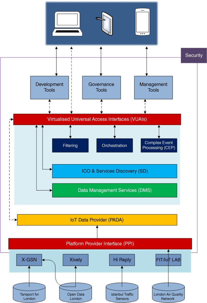
Figure 10.1 The VITAL platform architecture.
10.3.2 VITAL Prediction Module
Generally, most of the collected data in city data repositories can be considered as time series; hence, time series analysis (Gulacar, Yaslan and Oktug, 2016) or interpolation techniques are used (Dobre and Xhafa, 2014) for analysing them. On the other hand, one can also obtain feature vectors from sensor observations, and depending to the application domain, successful machine learning algorithms can be applied for classification, clustering, and regression applications. In order to predict sensor observations, regression algorithms can be used, where the aim is to find a continuous function between a dependent variable and one or more independent variables (Pan et al., 2013). Besides, regression relies on a loss function, which is generally the difference between the predicted value and the actual value to learn the best function, the one with least error. In this subsection, we will use the most common and successful regression models, such as support vector regression, regression trees, etc., for traffic sensor data prediction in Istanbul (Gulacar, Yaslan, and Oktug, 2016). We consider various representations of the feature vectors and their effects on performance as well.
The prediction module explained is an extension to the VITAL platform architecture given in Figure 10.1. The VITAL platform easily enables to extend services when the security issues are implemented. The extended prediction module and its VITAL integration are shown in Figure 10.2. As shown in the figure, the prediction module communicates with the VITAL security module and observes data via DMS and has core components that are listed below:
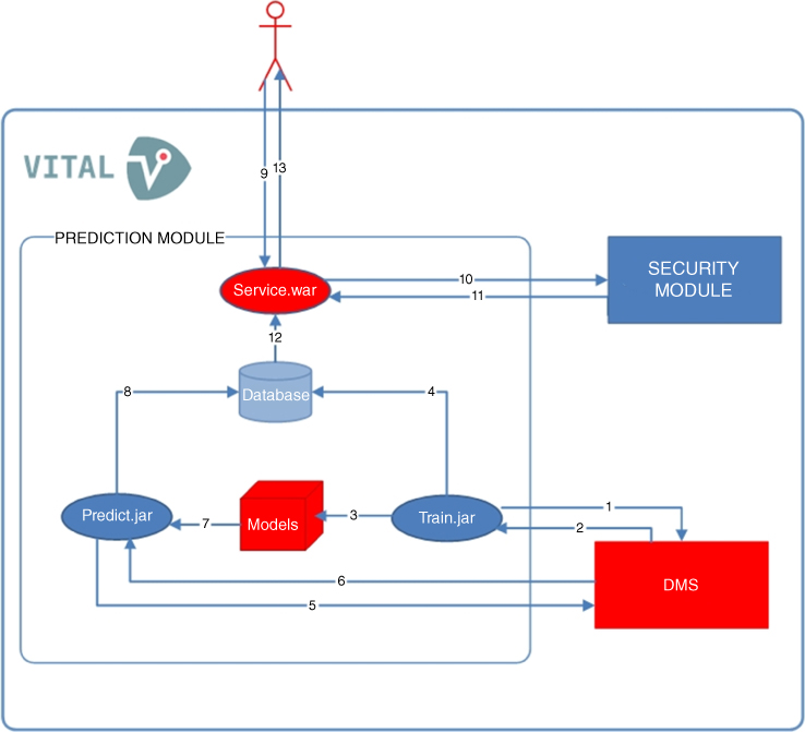
Figure 10.2 The VITAL prediction module extension.
Prediction module components:
- VITAL security module: Determines whether an access token is valid or not.
- VITAL DMS: Stores sensor observations, lists, etc.
- Service.war: Gets, controls, and responds to client requests.
- Database: Stores prediction results in MongoDB.
- Train.jar: Trains data in order to produce regression models and saves models. It is scheduled as working once every week.
- Models: Folder that includes all models created after training.
- Predict.jar: Gets data and makes prediction by using pickle. It is scheduled as working once every 15 minutes.
Communication between components (edges):
- Training data request: Send request DMS in order to get sensor observations for training.
- Training data response: Get sensor observations from DMS.
- Save model: Regression models created in training phase are saved into Models folder in order to reuse by Predict.jar.
- Weekly prediction results: Train.jar creates regression models. Additionally, it predicts weekly (long‐term) data and inserts into database.
- Observation request: Send request to DMS in order to get sensor observations.
- Observation response: DMS response that includes sensor observations.
- Get Model: Gets regression models for prediction.
- Insert prediction results: Insert prediction results to database.
- Client Request: Client must send request whose header includes vitalAccessToken and body includes the following item(s):
- Security request: Server.war sends request to VITAL/securitywrapper in order to determine whether vitalAccessToken is valid or not.
- Security response: VITAL/securitywrapper response whether vitalAccessToken is valid or not.
- Related prediction results: Asks prediction results from database according to user query.
- Prediction response: Prediction response is a list of nodes including the following items:
- city: PPI name
- sensor: sensor ID
- property: observation property
- value: predicted observation value
- prediction_time: shows when the module predicted that value
- minute_later: shows which prediction time mode (15 min., 30 min. ahead, or long‐term(999))
- predicted_time: shows for which time the module predicted that value.
In order to observe prediction results from the VITAL platform, one needs to implement the post method given in Table 10.2.
Table 10.2 VITAL Prediction Module Access Method.
| Query Predictions from Prediction Module | ||
| Description | This interface is used to query prediction results. | |
| Method | POST | |
| URL | PREDICTION_BASE_URL/prediction | |
| Request headers | Content‐Type | application/json |
| Cookie | vitalAccessToken | |
| Request body | Example { "sensors": [ "http://vital‐integration.atosresearch.eu:8280/hireplyppi/sensor/vital2‐I_ TrS_32Dir0" ], "city": "hireplyppi", "lt": "2016‐11‐23T15:34:00+00:00", "property": [ "Traffic" ], "gt": "2016‐11‐23T14:34:00+00:00" } |
|
| Response header | Content‐Type | application/json |
| Response body | Example [ { "predicted_time": "2016‐11‐23T15:30:00Z", "city": "hireplyppi", "property": "Traffic", "prediction_time": "2016‐11‐23T14:30:00Z", "sensor": "http://vital‐integration.atosresearch.eu:8280/hireplyppi/sensor/ vital2‐I_TrS_32Dir0", "value": 85, "minute_later": 60 } ] |
|
| Notes | • Request must include vitalAccessToken Cookie. • Request does not have to include “sensors,” “property,” “gt,” and “lt” items. |
|
10.4 A Use Case Employing the Traffic Sensors in Istanbul
Istanbul, with population of 14 million, is one of the most crowded metropolises in the world, and its 856‐kilometer‐long road network contains approximately 3 million cars (Gulacar, Yaslan, and Oktug, 2016). This huge amount of cars cause traffic jams on the complex road network of the city. Therefore, monitoring the traffic is crucial for management, and for this purpose, Istanbul Metropolitan Municipality (IMM) deployed many traffic speed sensors around the roads.
In this work, we used sensor observations from the D100 road, which connects the Asian part and the European part of Istanbul and has an airport at either end. The D100 road segment is shown in Figure 10.3. This data set contains approximately 30 million speed observations collected by 122 sensors located on the D100 road from Jan 1, 2014, to Dec 31, 2014. These observations are obtained from Autoscope Terra (image processing sensor), RTMS (Radar Sensor), Smart Sensor HD (Radar Sensor) type sensors which send observations every 1–2 minutes (Gulacar, Yaslan, and Oktug, 2016).
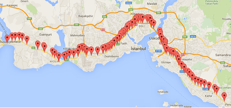
Figure 10.3 D100 road segment and deployed speed sensors.
10.4.1 Prediction Techniques Employed
In our previous work (Gulacar, Yaslan, and Oktug, 2016), we studied in detail the effects of using different feature vectors and clustering and regression methods on traffic speed prediction results. We determined that while the weather feature does not increase the prediction performance beyond our expectations, binary record time vectors increased the accuracy. Therefore, in this work we applied prediction methods on feature space that include previous speed observations and binary record time vectors. We also did extensive analysis on the data set employed. We showed that the observations of sensors at time t are strongly correlated with the observations of their neighbor sensors at time t – 30, as shown in Figure 10.4. In this experiment we aimed to find whether there is a relationship between the average values of sensor observations. Mostly, neighbouring sensors have relationship with the next sensor after 30 min. Thus this speed information is added as an extra feature in our predictions. Additionally, we analyzed the effect of adding neighbor sensor observation(s) to the feature vectors.
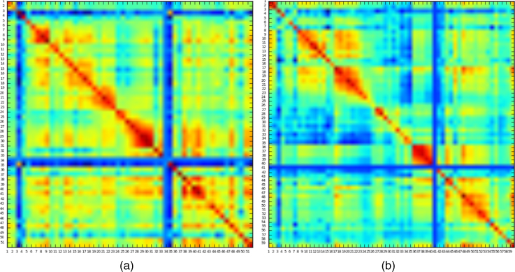
Figure 10.4 Neighbour sensor correlation: Correlation between speed observations at time t of sensor in the row and speeds at time t − 30 of sensor in the column. Sensors are sequential in direction from (a) Europe to Asia and (b) from Asia to Europe.
In this work, the clustering step is neglected since the module is compatible with a real IoT platform VITAL. While new sensors and/or PPIs can be added to the platform, determining a cluster is an extra burden for the platform. Besides, there is no significant differences between success of using clustering methods.
In the rest of this section, firstly, we describe data preprocessing operations. Then, constructions of feature vectors and normalization steps are described. Later, we describe training and test partitioning, and evaluation metrics are given. Finally, we give the applied regression methods and experimental results.
10.4.1.1 Data Preprocessing
In order to prepare data to create feature vectors, the following preprocessing operations are employed:
- 5‐min average data: We obtained the speed average data within 5 minutes in order to avoid high fluctuations of speed data.
- Neighbour sensor detection: The raw data did not contain any information about neighbouring sensors. Only sensor directions (Asia to Europe or vice versa) and sensor coordinates were available. Therefore, by using this information we detected neighbouring sensors.
- Missing data and sensor ignorance: Some sensors' data are ignored because of the following causes:
- ∘ Some of the sensors don't have coordinate information.
- ∘ Observations of some sensors cannot be retrieved in some months.
- ∘ Terminal sensors don't have neighbour sensors.
10.4.1.2 Feature Vectors
Let ![]() represent the speed of i‐th sensor at time
represent the speed of i‐th sensor at time ![]() .; in order to predict
.; in order to predict ![]() we construct the following feature vector for regression:
we construct the following feature vector for regression:
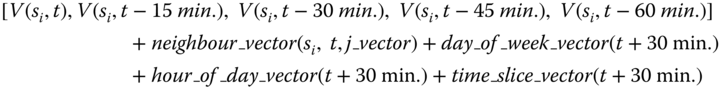
where:
- +: vector concatenation operator,
-
 : speed of i‐th sensor at time x,
 -
 : returns vector that includes speeds of
  sensor(s) that is/are neighbour(s) of
  at time t. For example,
 -
 returns
 -
 ,
, -
 : returns 7‐bit binary vector that represents day‐of‐week value of time x. For example,
  returns
 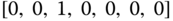 ,
, -
 : returns 24‐bit binary vector that represents hour‐of‐day value of time x. For example,
  returns a 24‐bit binary vector containing zeros except the leftmost 14‐th bit,
 -
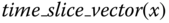 : returns 4‐bit binary vector that represents 15 min. time slice of hour value of time x. For example,
  returns
  .
.
After constructing the feature vectors, non‐binary features are normalized by using z‐score normalization. These feature extraction and model training and testing phases are given in Figure 10.5.
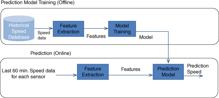
Figure 10.5 Prediction model training and online speed prediction for each sensor.
10.4.2 Results
Our experimental prediction results are obtained using various regression algorithms, namely: AdaBoost.R2 regressor (ADA; Solomatine and Shrestha, 2004), decision tree regressor (DTR; Breiman, Friedman, and Stone, 1984), Gradient boosting regressor (GBR; Friedman, 2002), K‐nearest neighbors regressor (KNN; Altman, 1992), kernel ridge regressor (KRR; Schölkopf, Luo, and Vovk, 2013), random forest regressor (RFR; Breiman, 2001) and support vector regressor with RBF kernel (SVR; Vapnik, 1995).
Adaboost regressor is an ensemble model and starts with fitting a model on the initial data set. Then, based on the error on the data set, it updates the selection probability of the samples and trains new prediction models on difficult examples.
Decision tree regressor is a hierarchical model that partitions the features based on a split measure such as mean square error. Decision trees are simple to interpret and handle both numerical and categorical variables.
Gradient boosting regressor is an ensemble model where several weak learners are learned on the residual of the previous models.
K‐nearest neighbors regressor estimates the target value of a data sample by calculating the average target values of the K nearest neighbors.
Kernel ridge regressor uses the least squares regression algorithm with regularization and applies Kernels functions.
Random forest regressor trains a number of decision tree regressors on various subsamples of the data set and combines their outputs to find the final result.
Support vector regressor is the generalization of support vector machines for regression problems. It aims to minimize the ɛ‐sensitive errors on the training set. Generally, a nonlinear kernel function is used to project initial data into a higher‐dimensional space.
Each regression algorithm is trained on a two‐month training set and evaluated on the upcoming test month using the aforementioned feature vectors. The training sets and test sets that are obtained using a sliding window is given in Figure 10.6.
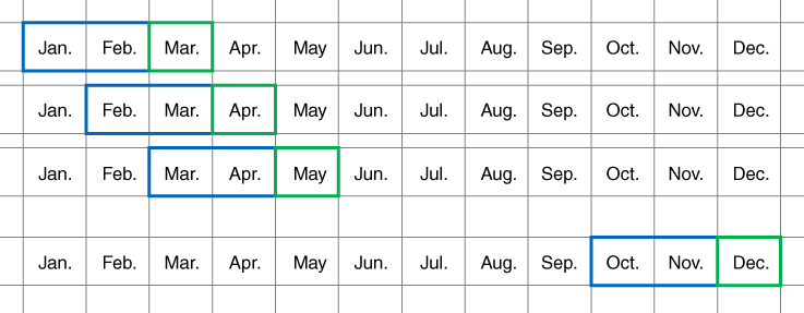
Figure 10.6 Training and test data set splitting. Two‐month training months (blue) and one‐month test (green) sets.
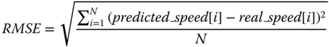
Experimental results are evaluated using root mean square error (RMSE):
10.4.2.1 Regression Results
The first experimental results are obtained without considering the neighbor sensors ![]() . These results for different regression methods are given in Table 10.3. The best accuracy is obtained with the kernel ridge regression method. On the other hand, the worst performance is obtained with the Adaboost.R2 regression algorithm.
. These results for different regression methods are given in Table 10.3. The best accuracy is obtained with the kernel ridge regression method. On the other hand, the worst performance is obtained with the Adaboost.R2 regression algorithm.
Table 10.3 RMSE for Different Methods without Neighbor Speed Information.
| ADA | DTR | GBR | KNN | KRR | RFR | SVR | |
| (10, 11) ‐> 12 | 16.85 | 15.62 | 14.03 | 15.21 | 13.91 | 14.38 | 14.77 |
| (9, 10) ‐> 11 | 17.89 | 16.82 | 15.33 | 16.41 | 15.21 | 15.65 | 16.02 |
| (8, 9) ‐> 10 | 17.95 | 17.10 | 15.38 | 16.63 | 15.26 | 15.75 | 15.71 |
| (7, 8) ‐> 9 | 17.13 | 17.59 | 15.84 | 16.48 | 15.64 | 16.28 | 16.18 |
| (6, 7) ‐> 8 | 17.02 | 15.94 | 14.07 | 15.20 | 14.01 | 14.47 | 14.59 |
| (5, 6) ‐> 7 | 18.54 | 16.39 | 14.59 | 15.67 | 14.71 | 15.06 | 14.70 |
| (4, 5) ‐> 6 | 16.57 | 15.36 | 13.54 | 14.60 | 13.49 | 14.03 | 13.92 |
| (3, 4) ‐> 5 | 15.20 | 13.78 | 12.18 | 13.39 | 12.12 | 12.55 | 12.74 |
| (2, 3) ‐> 4 | 15.37 | 13.84 | 12.20 | 13.42 | 12.21 | 12.59 | 12.85 |
| (1, 2) ‐> 3 | 15.19 | 13.70 | 12.06 | 13.02 | 12.06 | 12.39 | 12.64 |
| Regressor averages | 16.77 | 15.61 | 13.92 | 15.00 | 13.86 | 14.32 | 14.41 |
| Total average | 14.84 | ||||||
Next, we analyzed the effect of incorporating the previous sensor observations to the feature vector. The RMSE values obtained with the feature vector extended with the previous 1 sensor ![]() observations are given in Table 10.4. It can be seen from the table that the kernel ridge regression performs best, and incorporating the previous sensor observation slightly improved the performance.
observations are given in Table 10.4. It can be seen from the table that the kernel ridge regression performs best, and incorporating the previous sensor observation slightly improved the performance.
Table 10.4 RMSE for Different Methods with Observations of the Previous Sensor.
| ADA | DTR | GBR | KNN | KRR | RFR | SVR | |
| (10, 11) ‐> 12 | 16.78 | 15.61 | 13.90 | 15.02 | 13.75 | 14.25 | 14.57 |
| (9, 10) ‐> 11 | 17.49 | 16.79 | 15.12 | 16.18 | 15.02 | 15.42 | 15.73 |
| (8, 9) ‐> 10 | 17.87 | 17.36 | 15.45 | 16.48 | 15.17 | 15.77 | 15.57 |
| (7, 8) ‐> 9 | 17.11 | 17.56 | 15.63 | 16.26 | 15.44 | 16.07 | 15.98 |
| (6, 7) ‐> 8 | 16.86 | 16.02 | 13.97 | 15.01 | 13.88 | 14.35 | 14.36 |
| (5, 6) ‐> 7 | 18.91 | 16.89 | 14.87 | 15.71 | 14.86 | 15.33 | 14.72 |
| (4, 5) ‐> 6 | 16.69 | 15.78 | 13.70 | 14.63 | 13.58 | 14.11 | 13.98 |
| (3, 4) ‐> 5 | 15.11 | 13.95 | 12.21 | 13.39 | 12.14 | 12.56 | 12.74 |
| (2, 3) ‐> 4 | 15.63 | 14.29 | 12.39 | 13.51 | 12.36 | 12.77 | 12.94 |
| (1, 2) ‐> 3 | 15.40 | 14.00 | 12.13 | 13.02 | 12.09 | 12.50 | 12.63 |
| Regressor Averages | 16.79 | 15.82 | 13.94 | 14.92 | 13.83 | 14.31 | 14.32 |
| Total average | 14.85 | ||||||
The next experiment is obtained by incorporating the two previous sensor observations to the feature vector. The RMSE values obtained with the feature vector extended with the previous 2 sensor ![]() observations are given in Table 10.5. Note that incorporating the previous two sensors observations improves the prediction performance of all algorithms.
observations are given in Table 10.5. Note that incorporating the previous two sensors observations improves the prediction performance of all algorithms.
Table 10.5 RMSE for Different Methods with Observations of the Previous Two Sensors.
| ADA | DTR | GBR | KNN | KRR | RFR | SVR | |
| (10, 11) ‐> 12 | 16.47 | 15.61 | 13.85 | 15.01 | 13.72 | 14.20 | 14.56 |
| (9, 10) ‐> 11 | 17.64 | 16.83 | 15.15 | 16.23 | 15.05 | 15.47 | 15.80 |
| (8, 9) ‐> 10 | 17.88 | 17.29 | 15.40 | 16.45 | 15.20 | 15.75 | 15.61 |
| (7, 8) ‐> 9 | 17.01 | 17.65 | 15.72 | 16.35 | 15.49 | 16.16 | 16.08 |
| (6, 7) ‐> 8 | 16.64 | 16.10 | 14.06 | 15.08 | 13.91 | 14.48 | 14.43 |
| (5, 6) ‐> 7 | 18.54 | 16.65 | 14.61 | 15.52 | 14.67 | 15.06 | 14.61 |
| (4, 5) ‐> 6 | 16.54 | 15.63 | 13.49 | 14.39 | 13.39 | 13.95 | 13.78 |
| (3, 4) ‐> 5 | 15.21 | 14.07 | 12.26 | 13.41 | 12.17 | 12.65 | 12.75 |
| (2, 3) ‐> 4 | 15.63 | 14.17 | 12.33 | 13.46 | 12.30 | 12.70 | 12.91 |
| (1, 2) ‐> 3 | 15.45 | 13.97 | 12.09 | 12.96 | 12.01 | 12.47 | 12.55 |
| Regressor Averages | 16.70 | 15.80 | 13.90 | 14.89 | 13.79 | 14.29 | 14.31 |
| Total average | 14.81 | ||||||
The last experimental results are obtained by extending the feature vector the with the observations of the previous two sensors. The RMSE values obtained with the feature vector extended with the observations of the previous two sensors ![]() are given in Table 10.6. Although the result for KRR is better than the results given in Table 10.3, it is less than the results obtained with the feature set extended with the observations of the previous 2 sensor.
are given in Table 10.6. Although the result for KRR is better than the results given in Table 10.3, it is less than the results obtained with the feature set extended with the observations of the previous 2 sensor.
Table 10.6 RMSE for Different Methods with Observations of the Previous Two Sensor.
| ADA | DTR | GBR | KNN | KRR | RFR | SVR | |
| (10, 11) ‐> 12 | 16.37 | 15.64 | 13.81 | 14.91 | 13.65 | 14.13 | 14.44 |
| (9, 10) ‐> 11 | 17.59 | 16.78 | 15.04 | 16.12 | 14.96 | 15.35 | 15.62 |
| (8, 9) ‐> 10 | 17.87 | 17.73 | 15.52 | 16.42 | 15.19 | 15.94 | 15.54 |
| (7, 8) ‐> 9 | 16.95 | 17.62 | 15.61 | 16.23 | 15.41 | 16.09 | 15.96 |
| (6, 7) ‐> 8 | 16.36 | 16.26 | 13.93 | 14.94 | 13.80 | 14.34 | 14.23 |
| (5, 6) ‐> 7 | 18.91 | 17.11 | 14.82 | 15.60 | 14.90 | 15.25 | 14.68 |
| (4, 5) ‐> 6 | 16.66 | 15.79 | 13.65 | 14.52 | 13.54 | 14.10 | 13.91 |
| (3, 4) ‐> 5 | 15.31 | 14.29 | 12.35 | 13.50 | 12.27 | 12.72 | 12.83 |
| (2, 3) ‐> 4 | 15.58 | 14.58 | 12.58 | 13.65 | 12.54 | 12.95 | 13.12 |
| (1, 2) ‐> 3 | 15.41 | 14.29 | 12.25 | 13.10 | 12.18 | 12.65 | 12.69 |
| Regressor Averages | 16.70 | 16.01 | 13.96 | 14.90 | 13.84 | 14.35 | 14.30 |
| Total average | 14.87 | ||||||
Note that we also obtained experimental prediction results by extending the feature set using the following sensor observations ![]() ; however, none of these extensions performed better than the results obtained with the feature vector extended with the observations of the previous 2 sensor
; however, none of these extensions performed better than the results obtained with the feature vector extended with the observations of the previous 2 sensor ![]() . Therefore, we don't report them. The best performance for prediction is obtained with kernel ridge regression employing the feature vector extended with the observations of the previous 2 sensor
. Therefore, we don't report them. The best performance for prediction is obtained with kernel ridge regression employing the feature vector extended with the observations of the previous 2 sensor ![]() .
.
10.5 Conclusion
In this work, we summarized and compared most of the common smart city platforms with respect to the employed cloud support, communication protocols, authentication mechanisms, database systems, and prediction capabilities. Although, prediction has an important role in our daily lives, we see that only half of the platforms have prediction capabilities. We also introduce the VITAL smart city platform and its prediction module extension, which is implemented by employing the security mechanism in VITAL. The proposed module is evaluated for many traffic speed sensors deployed in Istanbul by Istanbul Metropolitan Municipality. We have compared the experimental prediction results obtained from various regression algorithms employing different feature vectors. It is observed that the best performance is obtained with kernel ridge regression employing the feature vector extended with the observations of the previous 2 sensor.
Acknowledgment
The tool and the use case presented in this chapter were developed with support from the EU Project with contract number CNECT‐ICT‐608682 and title “Virtualized programmable InTerfAces for smart, secure and cost‐effective IoT depLoyments in smart cities (VITAL).”
References
- Altman, N.S. 1992, ‘An introduction to kernel and nearest‐neighbor nonparametric regression’, The American Statistician, 46(3), pp. 175–185. doi: 10.1080/00031305.1992.10475879.
- Breiman, L., Friedman, J. and Stone, C.J. 1984, Classification and regression trees. New York, NY: Chapman and Hall/CRC.
- Breiman, L. 2001, Machine Learning, 45(1), pp. 5–32. doi: 10.1023/a:1010933404324.
- COMM 2016, European commission: CORDIS: Projects & results service: FI‐WARE: Future Internet core platform, viewed 5 December 2016, http://cordis.europa.eu/project/rcn/99929_en.html
- Cumulocity 2016, Cumulocity GmbH, viewed 5 December 2016, https://www.cumulocity.com
- Derhamy, H., Eliasson, J., Delsing, J. and Priller, P. 2015, ‘A survey of commercial frameworks for the Internet of things’, 2015 IEEE 20th Conference on Emerging Technologies & Factory Automation (ETFA). doi: 10.1109/etfa.2015.7301661.
- DeviceHive 2015, DataArt Solutions, viewed 5 December 2016, http://devicehive.com
- Digi 2016, Digi International Inc., viewed 5 December 2016, https://www.digi.com
- Digital Service Cloud 2015, viewed 2 November 2016, http://www.digitalservicecloud.com
- Dobre, C. and Xhafa, F. 2014, ‘Intelligent services for big data science’, Future Generation Computer Systems, 37, pp. 267–281. doi: 10.1016/j.future.2013.07.014.
- FIWARE 2011, viewed 5 December 2016, https://www.fiware.org
- Friedman, J.H. 2002, ‘Stochastic gradient boosting’, Computational Statistics & Data Analysis, 38(4), pp. 367–378. doi: 10.1016/s0167-9473(01)00065-2.
- GSN 2016, viewed 5 December 2016, https://github.com/LSIR/gsn/wiki
- Gulacar, H., Yaslan, Y. and Oktug, S.F. 2016, ‘Short term traffic speed prediction using different feature sets and sensor clusters’, NOMS 2016 ‐ 2016 IEEE/IFIP Network Operations and Management Symposium. doi: 10.1109/noms.2016.7503000.
- IoTgo 2014, ITEAD Intelligent Systems Co. Ltd., viewed 5 December 2016, http://iotgo.iteadstudio.com
- Kaa 2014, CyberVision Inc., viewed 5 December 2016, http://www.kaaproject.org
- Köhler, M., Wörner, D., and Wortmann, F. 2014, ‘Platforms for the internet of things – an analysis of existing solutions’, 5th Bosch Conference on Systems and Software Engineering (BoCSE).
- Mazhelis, O. and Tyrvainen, P. 2014, ‘A framework for evaluating Internet‐of‐Things platforms: Application provider viewpoint’, 2014 IEEE World Forum on Internet of Things (WF‐IoT). doi: 10.1109/wf-iot.2014.6803137.
- Mbed 2016, ARM Ltd., viewed 5 December 2016, https://www.mbed.com/en
- Mehta, Y., Pai, M.M.M., Mallissery, S. and Singh, S. 2016, ‘Cloud enabled air quality detection, analysis and prediction ‐ A smart city application for smart health’, 2016 3rd MEC International Conference on Big Data and Smart City (ICBDSC). doi: 10.1109/icbdsc.2016.7460380.
- Nimbits (n.d.), viewed 5 December 2016, http://bsautner.github.io/com.nimbits
- Pan, G., Qi, G., Zhang, W., Li, S., Wu, Z. and Yang, L. 2013, ‘Trace analysis and mining for smart cities: Issues, methods, and applications’, IEEE Communications Magazine, 51(6), pp. 120–126. doi: 10.1109/mcom.2013.6525604.
- Petrolo, R., Loscrì, V. and Mitton, N. 2015, ‘Towards a smart city based on cloud of things, a survey on the smart city vision and paradigms’, Transactions on Emerging Telecommunications Technologies, , p. n/a–n/a. doi: 10.1002/ett.2931.
- Pradhan, S., Dubey, A., Neema, S. and Gokhale, A. 2016, ‘Towards a generic computation model for smart city platforms’, 2016 1st International Workshop on Science of Smart City Operations and Platforms Engineering (SCOPE) in partnership with Global City Teams Challenge (GCTC) (SCOPE ‐ GCTC), . doi: 10.1109/scope.2016.7515059.
- RealTime.io 2016, viewed 5 December 2016, http://realtime.io
- Santander‐fiware 2016, Santander‐fiware/hackathon , viewed 5 December 2016, https://github.com/santander‐fiware/hackathon
- Schölkopf, B., Luo, Z. and Vovk, V. 2013, Empirical inference Festschrift in honor of Vladimir N. Vapnik. Berlin: Springer Berlin.
- SensorCloud 2016, LORD MicroStrain, viewed 5 December 2016, http://www.sensorcloud.com
- Solomatine, D.P. and Shrestha, D.L. 2004, ‘AdaBoost.RT: A boosting algorithm for regression problems’, 2004 IEEE International Joint Conference on Neural Networks (IEEE Cat. No.04CH37541). doi: 10.1109/ijcnn.2004.1380102.
- SiteWhere 2009, SiteWhere LLC, viewed 5 December 2016, http://www.sitewhere.org
- Strohbach, M., Ziekow, H., Gazis, V. and Akiva, N. 2015, ‘Towards a big data Analytics framework for IoT and smart city applications’, in Modeling and Processing for Next‐Generation Big‐Data Technologies. Springer Science + Business Media, pp. 257–282.
- TempoIQ 2016, viewed 5 December 2016, https://www.tempoiq.com
- Thinger.io 2016, viewed 5 December 2016, https://thinger.io
- Thingsquare (xxxxn.d.), viewed 5 December 2016, http://www.thingsquare.com
- ThingWorx 2016, PTC, viewed 5 December 2016, https://www.thingworx.com
- Vapnik, V.N. 1995, The Nature of Statistical Learning Theory.
- VITAL 2016, The VITAL Consortium, viewed 5 December 2016, http://vital‐iot.eu
- Vlahogianni, E.I., Kepaptsoglou, K., Tsetsos, V. and Karlaftis, M.G. 2015, ‘A real‐time parking prediction system for smart cities’, Journal of Intelligent Transportation Systems, 20(2), pp. 192–204. doi: 10.1080/15472450.2015.1037955.
- Wang, Y., Cao, G., Mao, S. and Nelms, R.M. 2015, ‘Analysis of solar generation and weather data in smart grid with simultaneous inference of nonlinear time series’, 2015 IEEE Conference on Computer Communications Workshops (INFOCOM WKSHPS). doi: 10.1109/infcomw.2015.7179451.
- Xively 2016, LogMeIn Inc., viewed 5 December 2016, https://www.xively.com