
12
Environmental Monitoring for Smart Buildings
Petros Spachos1 and Konstantinos Plataniotis2
1 School of Engineering, University of Guelph, Canada
2 Department of Electrical and Computer Engineering, University of Toronto, Canada
12.1 Introduction
Environmental monitoring describes the processes and activities that need to take place to characterize and monitor the quality of the environment. Indoor air quality (IAQ) refers to the quality of the air within and around buildings and structures. Environmental and IAQ monitoring is an important concern since it relates directly to the health and comfort of building occupants. Occupants of buildings with poor IAQ report a wide range of health problems, which are often called sick building syndrome (SBS) or tight building syndrome (TBS), building‐related illness (BRI), and multiple chemical sensitivities (MCS) (CCOHS (2013)).
Common issues associated with IAQ include improper or inadequately maintained heating and ventilation systems as well as contamination by construction materials (glues, fiberglass, particle boards, paints, etc.) and other chemicals. At the same time, the increase in the number of building occupants and the time spent indoors directly impact the IAQ (CCOHS ( 2013)). Everyday, people work in their offices or sit on meeting rooms where the quality of the air can affect not only their performance but also their health.
There are many sources of indoor air contaminants:
- Carbon dioxide (
 ), perfume, and tobacco smoke, which come from building occupants.
 - Dust and gases from building materials.
- Toxic vapors and volatile organic compounds (VOCs) from workplace cleaners.
Some of these pollutants can be created also from indoor activities such as smoking and cooking. IAQ problems are more prevalent in indoor infrastructures such as houses, offices, and schools (EPA (2014)). It is necessary to develop of an accurate system for environmental and IAQ monitoring system that can be used in the current buildings as well as the smart buildings of the near future.
Traditionally, environmental monitoring includes a small number of expensive and high‐precision sensor units. The units are placed in fractions of the building and monitor the quality of the air. Collected data are retrieved directly from the equipment at the end of the experiment after the units have been recovered. The limited number of sensor units, due to their cost, along with the lack of correlation in real‐time data collection is the main drawback of this approach.
Recent progress in wireless communication and sensor technologies can provide better, real‐time monitoring of the environmental condition through smart sensors with lower cost and wireless capabilities. Every day more computer‐based devices are connected to the Internet. Most of these devices have at least one sensing unit, creating opportunities for direct integration between the physical world and computer‐based systems. This is the idea behind the Internet of things (IoT), a development of the Internet in which everyday objects have network connectivity, allowing them to send and receive data (Fang et al. (2014)).
In the near future, wireless sensor networks (WSNs) are expected to be integrated into the IoT and consequently to smart cities and smart buildings (Jin et al. (2014b), Bellavista et al. (2013a)). The sensing infrastructures have a major role in the IoT and great research opportunities. Sensor nodes can join the Internet dynamically and use it to collaborate and accomplish their tasks. The future Internet, designed as an IoT, is foreseen to be a world‐wide network of interconnected objects uniquely addressable, based on standard communication protocols. Similar to the IoT, sensors will have a crucial role in smart cities (Jin et al. (2014a), Cardone et al. (2013)). Green cities, which span from urban wildlife initiatives to urban agriculture and green transport networks, citizen sensing, and smart cities projects are emerging that attempt to realize improved sustainability through greater urban connectivity.
At the same time, the sensor node market continues to grow rapidly, as the cost to build custom nodes decreases due to technology scaling. Moreover, the use of embedded sensors in smartphones, phablets, tablets, and mobile devices has enabled a number of popular applications (Sheng et al. (2013), Lathia et al. (2013)). Advances in technology, engineering, and materials science have opened the door for increasingly sophisticated sensors to be used in environmental monitoring research. The flexibility of sensor nodes permits fast time‐to‐market, which is crucial in the development of new sensor network applications. From the cost perspective, embedded sensor in mobile devices are already superior to application‐specific hardware. As an example, an indoor positioning system (IPS), which based on magnetic and other sensor data or a network of devices is more flexible, secure, and inexpensive in comparison to the global positioning system (GPS) (Shin et al. (2012)).
Environmental monitoring serves a vital scientific role by revealing long‐term trends that can lead to new knowledge and better understanding of the environment. WSNs are ideal systems for environmental monitoring. Inch scale sensors with low cost can be deployed over large areas to collect data. The use of WSNs for monitoring applications covers a wide area of the environmental monitoring (Oliveira and Rodrigues (2011), Othman and Shazali (2012)), from air and water quality monitoring to rain forest and biodiversity monitoring. Sensor nodes are the elementary components of any WSN, and they can provide many functionalities including signal conditioning and data acquisition, temporary storage for the data, data processing, analysis of the processed data, self monitoring (e.g., supply voltage), scheduling, receipting and transmission of data packets, and coordination and management of communications and networking.
However, they also pose a number of challenges, with survivability being one of the most crucial. The lifetime of any individual node and as a consequence, of the whole network, is solely decided by how the limited amount of energy is utilized. Energy harvesting can alleviate this problem. Self‐powered WSNs provide the possibility of very long sensor node lifetimes while their deployment would have the least impact on the existing infrastructure. Moreover, with a carefully designed routing mechanism (Al‐Karaki and Kamal (2004)), the total network lifetime can be extended compared with traditional battery‐powered WSNs.
The objective of this chapter is to introduce an environmental monitoring system for smart buildings. It focuses on the requirements and challenges of a real‐time monitoring system for ![]() in a smart building and describes a prototype that was developed to meet the needs of the application.
in a smart building and describes a prototype that was developed to meet the needs of the application.
The rest of the chapter is organized as follows: Section 12.2 gives a brief description of the wide area of WSN‐monitoring applications. Section 12.3 introduces the design goal along with the requirements and challenges of the specific application. Section 12.4 introduces the proposed architecture for the proposed system, followed by Section 12.5 with the experimental results and discussion. Section 12.6 concludes the chapter.
12.2 Wireless Sensor Networks in Monitoring Applications
WSNs are a promising solution for a plethora of monitoring applications due to their low cost and low power characteristics (Akyildiz et al. (2002), Yick et al. (2008)). They are used from general surveillance (Ghataoura et al. (2011)) to structural health monitoring in buildings (Torfs et al. (2013)) and highway bridges (Sazonov et al. (2009)).
In recent years, environmental‐monitoring applications have grown rapidly in areas such as agricultural monitoring (Kays et al. (2011), Bencini et al. (2009)), habitat monitoring (Mainwaring et al. (2002)), and climate monitoring (Martin et al. (2014)). The IoT along with the smart cities concept (Zanella et al. (2014), Spachos et al. (2015)) brings new areas for deployment for environmental monitoring. At the same time, it also brings different requirements and challenges.
Environmental‐monitoring applications can be broadly categorized into outdoor and indoor monitoring (Arampatzis et al. (2005)). In outdoor‐monitoring applications usually the WSN is deployed in a remote location and harsh environment with limited energy sources. Outdoor‐monitoring applications include chemical hazard detection (Jan et al. (2010)) and air pollution detection (Suganya and Vijayashaarathi (2016)) with challenges such as weather condition and energy limitations. In indoor‐monitoring applications, the WSN is deployed in an indoor environment along with others that might use the wireless channels. Indoor‐monitoring applications include building and office monitoring (Torfs et al. ( 2013)) and parking space detection (Corral et al. (2012)) with challenges such as the absence of accurate location techniques and the interference from other wireless communication applications.
Environmental condition monitoring in homes have been examined in Kelly et al. (2013). The authors proposed a framework to monitor temperature, humidity, and light intensity, which is based on a combination of pervasive distributed sensing units, information system for data aggregation, and reasoning and context awareness. The reliability of the sensing information is encouraging.
Recently a number of systems have been proposed for carbon dioxide monitoring (Spachos and Hatzinakos (2016)). In Yang et al. (2013), a remote carbon dioxide concentration monitoring system is developed. The system reports geological ![]() , temperature, humidity, and light intensity of the outdoor monitoring area. Similarly, in Mao et al. (2012) an urban
, temperature, humidity, and light intensity of the outdoor monitoring area. Similarly, in Mao et al. (2012) an urban ![]() monitoring system is presented. The system operates outdoors at an urban area around 100 square kilometers.
monitoring system is presented. The system operates outdoors at an urban area around 100 square kilometers.
Indoor environments can pose different challenges to a monitoring system. Indoor and outdoor air quality monitoring through a WSN is presented in Postolache et al. (2009). Each node has an array of sensors, and it is connected to the central monitoring unit either hardwired or wirelessly. In Kim et al. (2014), a real‐time indoor air quality monitoring system is proposed. The system has seven sensors monitoring seven different gases. In Jelicic et al. (2013), a system with aggressive energy management at the sensor level, node level, and network level is presented. The system detects volatile organic compounds (VOCs) and CO and saves energy through context‐aware adaptive sampling. A low‐power ZigBee sensor network to monitor VOCs pollution levels in indoor environments is proposed in Peng et al. (2015). The network consists of end device sensors with photoionization detectors and routers.
12.3 Application Requirements and Challenges
Environmental monitoring for smart buildings has a number of requirements while it poses a few constraints and challenges. The monitoring area and the application scenario affects both the requirements and the challenges while the monitoring target, the sampling rate, and the overall deployment cost are some of the parameters that should be considered in the design decisions of the system. At the same time, wireless network coexistence and dynamic environment changes are challenges that any proposed solution should overcome.
12.3.1 Monitoring Area
Many of the design decisions are affected by the selection of the monitoring area. When the requirements and challenges of the monitoring area are well defined, the design decisions for the proposed monitoring system can be optimized. Most of the time, environmental monitoring refers to the air pollution (Boubrima et al. (2017)) and general environment conditions, so the monitoring system can be deployed either indoors or outdoors. The monitoring area can be further categorized to simple or complex based on the surrounding area.
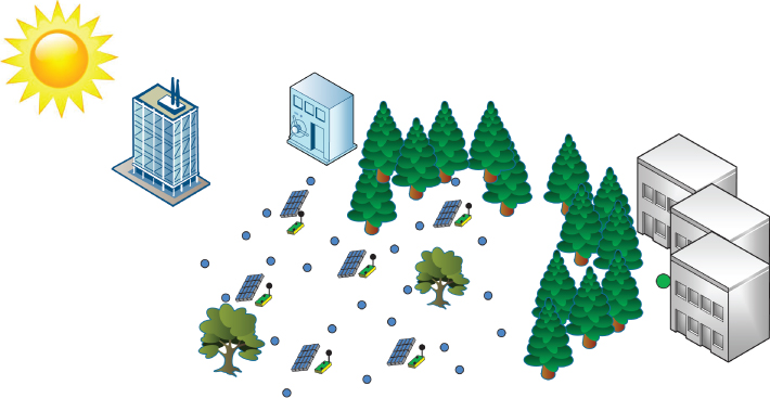
Figure 12.1 An outdoor self‐powered wireless sensor network.
At an outdoor‐monitoring system, the nodes are deployed outside in an open area, similar to the one shown in Figure 12.1. In such monitoring area, the communication between the nodes is easier when line of sight (LoS) between the nodes is possible. A proper deployment of the nodes can minimize the interference and enhance the communication between neighboring nodes that are within LoS. Another advantage is the potential usage of renewable energy resources such as wind and solar energy. The nodes can use these resources to extend their operation lifetime and consequently extend the total network lifetime. Solar panels and wind turbines can be used for energy harvesting in order to extend the network lifetime significantly. Moreover, without the need of battery replacement, the system can work unattended in remote locations and for long periods.
An outdoor‐monitoring system can also make use of the Global Positioning System (GPS) for more accurate target detection and optimal communication. Nodes can have access to GPS information not only for target tracking but also for route decision making. There are a number of routing protocols in the literature that can optimize the energy consumption, if the location of the nodes in the network is known (Pantazis et al. (2013), Zorzi and Rao (2003), Maihofer (2004), Spachos and Hantzinakos (2014), Spachos et al. (2012)). However, the use of GPS will increase not only the energy requirements for each monitoring node, but it will also increase the cost per node and the total system cost.
The surrounding area can be categorized further in simple and complex. A monitoring system deployed in an isolated area can use wireless communication with minimum or no interference with other networks. The nodes deployment is easier while most of them will be in LoS. On the other hand, the deployment of a monitoring system at an urban environment is more complicated (Bellavista et al. (2013b)). The available space and location for the nodes is limited while the network has to overcome requirements such as the proper placement of the sensors in comparison with other devices in the area and challenges, such as the communication between the nodes through noise and overcrowded channels and frequencies. Moreover, these networks are characterized by multi‐hop lossy links while the nodes are exposed to weather conditions.
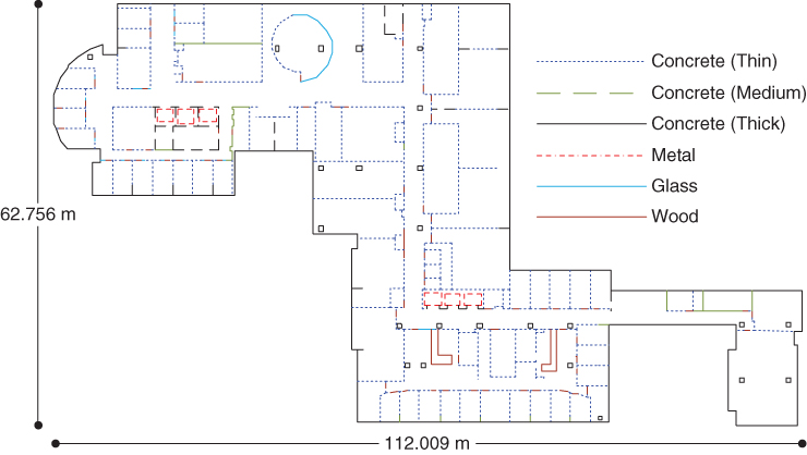
Figure 12.2
The  floor of Bahen Centre for Information Technology building at the University of Toronto, Canada. It is a complex indoor environment with a number of classrooms, offices, and open areas. The materials are categorized into six types: thin, medium, and thick concrete, metal, glass, and wood. Each material has a different effect on the wireless signals.
On the other hand, an indoor‐monitoring system would have its unique requirements and pose different challenges than an outdoor system. One of the main challenges of the indoor environment for wireless communication is the non‐line‐of‐sight (NLoS) problem. The LoS path can be blocked, and the communications are conducted through reflections and diffractions (Spachos et al. (2011)). Multiple contributions between communicating nodes are constructed by reflections, transmissions and, diffractions on the building structures. At the same time, energy harvesting is more challenging (Chirap et al. (2014), Yu and Yue (2012)) while the associated cost can be high.
Regarding the location of the nodes, it should be determined through different techniques (Guo et al. (2010), Hood and Barooah (2011)), since GPS is not available. This increases the complexity of the overall system design, especially, if the nodes are mobile and they need to know their location while they are moving within the monitoring area.
The monitoring area can be simple, inside an office with many open areas, or complex, covering the floor of a building, similar to the one shown in Figure 12.2. In this area, the materials have been categorized into six types: thin, medium, and thick concrete, metal, glass, and wood. Every material type has different characteristics that have different effects on the wireless communication between the nodes. This is a good example of a complex indoor environment and presents a lot of scatterers and obstacles such as walls, pillars, wooden doors, etc. These are of great influence when the radio links in such areas are examined. An efficient monitoring system has to take into consideration those objects to correctly predict the communication link availability in the area. Attenuation, distortion, and noise increase the complexity of the system for reliable communication.
12.3.2 Application Scenario and Design Goal
Along with the monitoring area, the application scenario is another important factor of an efficient monitoring system. In this work, a real‐time monitoring system for the concentration of ![]() at a whole floor of a crowded university building is developed. A number of wireless sensor nodes with gas leak detection capabilities and simple relay nodes are deployed in the monitoring area. The wireless sensor nodes are equipped with a gas sensor module and a wireless transmission module. The data from the sensor module are passed to the transmission module. The transmission module will forward all the necessary data to the control room, through the relay nodes. The relay nodes have only communication capabilities. Both the sensor units and the relay nodes are powered with batteries.
at a whole floor of a crowded university building is developed. A number of wireless sensor nodes with gas leak detection capabilities and simple relay nodes are deployed in the monitoring area. The wireless sensor nodes are equipped with a gas sensor module and a wireless transmission module. The data from the sensor module are passed to the transmission module. The transmission module will forward all the necessary data to the control room, through the relay nodes. The relay nodes have only communication capabilities. Both the sensor units and the relay nodes are powered with batteries.
The floor has rooms of different sizes (offices, laboratories, meeting rooms) and number of occupants while the areas have different materials, as discussed in the previous section. Many people spend most of their time inside the building, either in their offices or in meeting rooms. The quality of the air along with the environmental conditions in the room can affect not only their health but also their general performance. General solutions that are applied to every room in the building, such as average room temperature, are not efficient while most of the time the temperature of an area of the floor is considered. The lack of real‐time data of the condition inside each room decreases the efficiency of these systems while some times it ends up being more costly.
During the day, the number of people in the rooms changes; hence, the quality of the air changes. A smart heating, ventilation, and air conditioning (HVAC) system should take into consideration these parameters and take different actions in every case. An efficient environmental monitoring system should collect useful data from each room in the building, forward the data to a control room, and finally take actions toward the improvement of the environment in each room separately. For instance, the conditions in a meeting room with 10 people should be different from a similar meeting room with more occupants or with no occupants at all. The air conditioning system of an office should change based not only on the temperature of room but also on the quality in the air. Dynamic changes in the environment, such as gases from cooking, an open window, or an increase of the number of occupants in the room, need time to alter the temperature of the room, which is usually the trigger factor of the air conditioning. An environmental monitoring system for a smart building should be aware of the dynamic changes and respond as soon as possible to these changes.
The proposed system was deployed at a region of the ![]() floor of Bahen Centre for Information Technology at the University of Toronto, shown in Figure 12.3. The offices that were used are for researchers, students, and visitors and a meeting room was used as well. None of the offices or the meeting room have windows and all are connected to the same ventilation system. During day time, each office has either one or two people working, while more people can come and stay in each room. The meeting room can have between 14 and 18 people.
floor of Bahen Centre for Information Technology at the University of Toronto, shown in Figure 12.3. The offices that were used are for researchers, students, and visitors and a meeting room was used as well. None of the offices or the meeting room have windows and all are connected to the same ventilation system. During day time, each office has either one or two people working, while more people can come and stay in each room. The meeting room can have between 14 and 18 people.
The main focus of this work is to improve the indoor air quality of these rooms. The proposed solution will work along with the existing HVAC system and improve its efficiency. At the same time, the privacy of the occupants is also considered; hence, no cameras or any other visual sensors were used to count the number of the occupants in the room or decide the existence of people in the monitoring area.
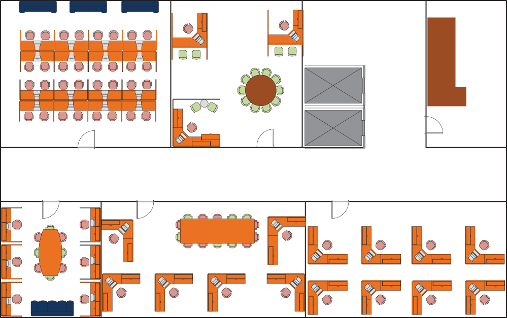
Figure 12.3
A region of the  floor of Bahen Centre for Information Technology building at the University of Toronto, Canada, that was used for experimentation.
12.3.3 Requirements
Following the described application and the monitoring area, the proposed system needs to meet the following requirements.
12.3.3.1 Sensor Type
The first requirement involves the proper selection of the sensor type. For indoor air quality monitoring there are three types of gas sensors that can be used:
- Electrochemical
- Optical
- Metal Oxide Semiconductor (MOS)
Electrochemical sensors can be used to monitor several toxic gases such as carbon monoxide and oxides of nitrogen. The gas goes through a chemical reaction, producing a current. The current is directly proportional to the concentration of the gas in the environment. Electrochemical sensors have high sensitivity, with low energy requirements. However, they have relative short lifetimes, their response times can be long, while their costs and their sizes vary.
Optical sensors can be used for carbon dioxide gas determination with long lifetime, high sensitivity, and low energy consumption. Also, the warm up and the response time of optical sensors is short. However, the cost of the sensors is high.
A MOS sensor is a popular choice due to the low cost, the small size, and the long lifetime. The warm up time of these sensors is long, but the response time is short. Most of the indoor air quality sensors belong to the MOS type. The proposed system will use MOS sensors due to their advantages in comparison with the other two sensor types for the selected application and the monitoring area.
12.3.3.2 Real‐Time Data Aggregation
Real‐time data aggregation is an important requirement. The monitoring data should reach the control room on time and after the necessary processing, the optimal condition should be applied to each room of the smart building. There is an upper bound limit on the transmission delay of the data, after which the data are not useful any more. This requirement poses significant challenges on the selection of the routing protocol. A routing protocol should not only try to minimize the energy requirement of the wireless nodes but also deliver the data on time for further processing.
12.3.3.3 Scalability
The proposed system should cover a wide area with hundreds or even thousands of nodes. It is necessary for any proposed solution to prove that is well suited to large scale WSNs. The system scalability and node mobility are important requirements. A high number of sensors can be installed in a building while some of them might need to be placed in other parts of the building after a certain time. The framework should be scalable to include more sensors while it should also be able to provide connectivity to mobile nodes which change location over time.
At the same time, the number of sensors in the monitoring area is important. It is affected by the reliability and energy requirements of the sensor, the sensing area, and the cost. The more reliable and accurate are the sensor readings, the less sensors are needed to cover the monitoring area while the sensor calibration is faster. Similarly, when the coverage area of a sensor is large, the monitoring area can be covered with a small number of nodes. However, hardware malfunction and dynamic changes in the communication between nodes can affect the overall system performance. In general, as the number of sensors increases, the system accuracy and reliability increases as well. On the other hand, as the number of sensors increases, the cost and the network traffic increases, and more complex algorithms are necessary for reliable communication.
Another important aspect of the network scalability and the number of required nodes is the placement of them at the monitoring area. A detailed study of the monitoring area can help improve the sensor placement, minimize their number, and optimize the communication among them. For instance, the distance between the sensor and an open window or the ventilation system can affect the data. A placement of the sensor away from factors that can affect its readings would increase the reliability of the system.
12.3.3.4 Usability, Autonomy, and Reliability
The monitoring devices should be easy to use, small in size, and low cost. Each monitoring node should be able to join or leave the network at any time without the need of a special configuration. This would minimize the need for administration and maintenance. At the same time, the size of the nodes is important in order to be placed easily in a complex indoor environment. The cost of the device will affect the overall design cost of the proposed solution and many of the requirements, as described in the previous section.
The nodes should also be able to work autonomously. Batteries must be able to power the nodes during the whole deployment. Due to the wireless communication and the associated energy consumption, the network has to be efficient energy‐wise, even if a renewable source of energy is used. This also affects the routing protocol. The protocol should turn off the radios periodically while it has to make sure that the remaining active nodes are able to cover all the monitoring area.
Moreover, the network should be able to perform simple operations to prevent unexpected crashes or general hardware problems in order to minimize the need for maintenance. End user maintenance should be avoided, since they may not have networking knowledge or because the areas of interest are most often remote. Achieving reliability is difficult because packet losses are more likely to happen during high network traffic, which are at the same time the most interesting episodes for data analysis.
12.3.3.5 Remote Management
The proposed system will be installed in a wide area while the nodes will be placed in locations that are hard to be visited regularly. Hence, remote access is necessary to operate, manage, and reprogram the nodes and to configure the whole system, regardless of manufacturer.
These are the minimum requirements for an efficient environmental‐monitoring system. When the application changes, some other requirements come into consideration.
12.3.4 Challenges
Environmental monitoring in smart buildings faces a number of challenges. The more specific are the requirements of the system, the better estimation can be made regarding the expected challenges.
12.3.4.1 Power Management
For long‐term operation of the system, an efficient power management approach should be followed. Environmental monitoring in smart buildings is used to minimize the energy requirements. Hence, the proposed system should have minimum energy requirements and be able to operate for long time. The energy footprint of the system should be small and, as a consequence, the energy consumption of the monitoring nodes should be low.
Power management also affects the routing protocol and the general design of the prototype. The protocol should minimize the communication between the nodes while it should force an energy efficient duty cycle scheme for the nodes. In this way, energy can be saved in the nodes, and the overall lifetime of the network can be extended.
The overall design of the system should take into consideration the power management. Although different sensors can improve the data accuracy, the energy requirements of the sensor is important. Since the application is specific and the requirements are clear, sensors that meet the requirements and have low energy consumption should be selected.
12.3.4.2 Wireless Network Coexistence
Another important challenge for every indoor monitoring systems is wireless network coexistence. The monitoring system is deployed in an area where there are other wireless connections. The environment of a building has a number of other wireless transmissions between laptops, desktops, smart phones, routers, etc. Especially the unlicensed band of 2.4 GHz is overcrowded. Devices that operate at the same place over the same spectrum need to have mechanisms to minimize collision, get access, and share the medium. Spectrum availability detection, interference mitigation, and spectrum sharing are requirements that every wireless system needs to properly address.
12.3.4.3 Mesh Routing
The mesh networks topologies can both provide multi‐hop and path diversity. A routing protocol to support multi‐hop mesh network is crucial, which must take into account the very limited features of the network. The routing protocol should also support the time and delay requirements of the application.
12.3.4.4 Robustness
The network must account for a lot of problems such as poor radio connectivity or hardware failures. The use of any protocol requiring an initialization phase to be performed synchronously by all nodes is thus inconceivable.
12.3.4.5 Dynamic Changes
Another challenge is the dynamic changes in the environment. In smart buildings, people are moving between rooms, and they can temporarily block the signals. At the same time, smart mobile devices also move between rooms, changing the interference and the link availability over time. The proposed system should be able to adopt to dynamic changes and transmit the information to the control room.
12.3.4.6 Flexibility
Nodes can join or leave the network based on the application needs for coverage in different areas. For instance, more nodes can be placed in a meeting room during a meeting while nodes can be removed from offices that are not used any more. It is crucial for the nodes to be able to automatically detect their neighborhood and minimize the need for reconfiguration.
12.3.4.7 Size and cost
The nodes should be small in size in order to be flexible in their placement in the area. Also, nodes might need to be placed in different rooms; hence, the node size is important to move the nodes around. Finally, all the requirements and challenges should be addressed with the minimum cost. The necessary hardware components and their cost should be minimum, especially for large‐scale deployments.
12.4 Wireless Sensor Network Architecture
In this section, the general framework that was used in the proposed system is described, followed by a brief description of the hardware components and the data processing.

Figure 12.4
System framework of indoor  monitoring system.
12.4.1 Framework
The system framework is shown in Figure 12.4. It has three core units: the wireless monitoring nodes, the wireless ad hoc network, and the control room. The implementation of each unit is based on the specific application; however, some minor modification can make the framework applicable to other environmental monitoring systems with similar principles. The core units have the following principles:
- Wireless monitoring nodes: This is the main sensor unit. A number of sensors for environmental monitoring can be connected to a transmission node. The transmission node is necessary to have a radio module in order to forward the data to the main wireless ad hoc network toward the control room. A low‐cost and low‐energy microcontroller can be used at the sensor unit for the initial filtering of the sensor data before the transmission. The monitoring nodes can be placed in different locations, and their location can change after the initial network configuration while more nodes can join the network or nodes can leave the network. It is important for the monitoring node to be flexible in placement and able to cope with dynamic changes. The nodes are powered with batteries while the developed prototype can also be powered through solar panels and store energy in rechargeable batteries (Spachos and Hatzinakos (2014)).
- Relay nodes: The relay nodes are used to provide connectivity between the sensor nodes and the control room. The relay nodes form a mesh network with a number of multi‐hop connections toward the destination. They have radio modules similar to the modules at the monitoring nodes, and they implement the routing protocol. The next node selection and the spectrum selection and sharing decision is taking place in the relay nodes. If storage is available at the relay nodes, then they can also store packets. However, the cost of the relay nodes should be lower than the cost of the monitoring nodes while they also need to be able to join and leave the network dynamically. The relay nodes are also powered with batteries, but their power requirements are lower than the monitoring nodes, since there is no sensor unit attached to the relay nodes.
- Control room: Main data processing, aggregation, and storage is taking place at the control room. The control room is at a remote location and can communicate with the monitoring nodes through the relay nodes. After collecting the monitoring data, the control room makes a decision about the environmental conditions in each room of the building. These decisions are related with the HVAC operation to improve the air quality in each room separately.
12.4.2 Hardware Infrastructure
The selection of the necessary hardware components should follow the requirements and the challenges, as described in previous sections, and also follow the main principles of the general framework. The introduced testbed has the following hardware components:
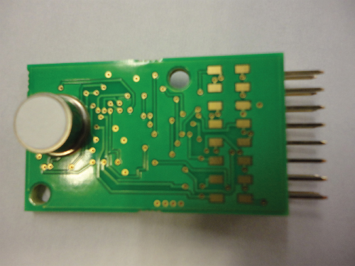
Figure 12.5 iAQ‐2000 sensor.
-
Sensor: The iAQ‐2000 carbon dioxide (
 ) sensor was used. iAQ‐2000 is a cost‐effective solution to accurately monitor the air quality of an indoor environment (CO2Meter). This sensor communicates using the RS‐232 communication protocol and consumes 46 mW of power while active, making it ideal for long‐term monitoring applications. The monitored
  levels are reported in a parts‐per‐million (ppm) value, which can be correlated to the air quality of an indoor environment. The iAQ‐ 2000 sensor is shown in Figure 12.5, and Table 12.1 shows the sensor specifications.
 -
Microcontroller and radio module. The OPM15 development board by RapidMesh was used as the main communication board (OMESH Networks). The OPM15 provides wireless capabilities for a network through its opportunistic wireless mesh radio. This low‐power device (41 mW during active cycle) is designed for low bandwidth applications. The microchip PIC18F26K22 programmable microcontroller enables networks to be quickly developed through open‐source C‐based applications. As well, the OPM15 is easily interfaced to additional components through SPI, I2C, or RS‐232 and has multiple free analog and digital ports available. The microcontroller along with the radio module is shown in Figure 12.6, and Table 12.2 shows the specification of the board.
Table 12.1 iAQ‐2000 specifications. Type MOS Substances detected  ,
,  ,
,  , Alcohols, Ketones, Organic acids, Amines, Aliphatic hydrocarbons, Aromatic hydrocarbons
Power supply 
Power consumption 
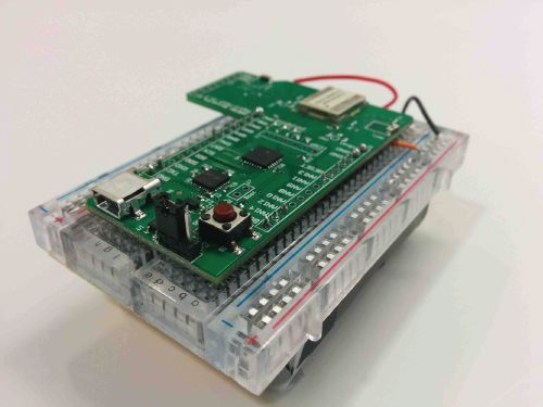
Figure 12.6 OPM
 relay node.
Table 12.2 OPM
 specifications.
Radio range 
Frequency range 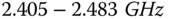
Channels 3 Bandwidth (per channel) 
Receiver sensitivity 
Transmitting power 
Power supply 
Power cons. (Sleep) 
Power cons. (Work) 
-
Power Converter
A prototype multifunctional power converter was used (Spachos and Hatzinakos (2015)). The assembly kit is show in Figure 12.7(a), and the circuit is shown in Figure 12.7(b). The prototype provides an all‐in‐one solution to power management and interfacing requirements between common hardware components. The prototype is capable of boosting and regulating an input voltage to a fixed 5V, has a built‐in shutoff to protect the battery source from over‐draining, is capable of recharging a lithium polymer (LiPo) battery with the aid of an energy harvesting device, and provides terminals to access the input power source's voltage. A toggle switch also enables the power to be solely drawn from an energy‐harvesting device instead of a LiPo battery.
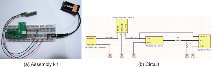
Figure 12.7 The indoor version of the prototype with (a) the assembly kit of the monitoring board, where a sensor unit is connected to a radio module through (b) a simple electric circuit.
12.4.3 Data Processing
An important part of the monitoring system is the data processing. The collected data are not of equal importance while sometimes it might be corrupted due to unreliable readings. It is necessary that an initial processing takes place at the radio module, before data transmission. The module processes the data collected from the sensor and transmits only the necessary information to the destination. In this way both the bandwidth and energy are saved. The system minimizes useless data transmissions, minimizing the traffic in the network and the energy consumption per node. The data is transmitted into packets. The data is processed and stored at the control room.
12.4.3.1 Noise Reduction, Data Smoothing, and Calibration
One of the major problems of using low‐cost MOS sensors is their unreliable readings. The sensors may report unreliable or corrupted data for a few readings. The sensor unit should decide whether the data are due to sensor malfunction or failure or there is an event in the area. This task should take place at the sensor node before the data transmission.
To reduce the sensor noise, a mobile sensor was used, similar to (Tsujita et al. (2004)). The mobile node moves in each of the monitoring rooms once every hour. The mobile node is equipped with the same sensor as the sensor units. The mobile node compares its readings with the readings reported from the different sensors in every room, for one minute. If the readings are close, the mobile sensor moves to the next sensor unit. If the sensor readings are within ![]() from the mobile sensor reading, the mobile sensor informs the control room for the necessary calibration. The calibration can take place remotely through the configuration at the control room. When the difference between the sensor unit and the mobile sensor is greater than the threshold above, there might be a need to replace the sensor node, and the system administrator needs to check the sensor on the site. The mobile node periodically updates the sensor units with the expected values according the previous levels in the area. This is important for the sensor units to detect potential outliers that can occur for a few readings.
from the mobile sensor reading, the mobile sensor informs the control room for the necessary calibration. The calibration can take place remotely through the configuration at the control room. When the difference between the sensor unit and the mobile sensor is greater than the threshold above, there might be a need to replace the sensor node, and the system administrator needs to check the sensor on the site. The mobile node periodically updates the sensor units with the expected values according the previous levels in the area. This is important for the sensor units to detect potential outliers that can occur for a few readings.
To identify outliers and remove them from the measurements, a smoothing algorithm is also followed. When a random spike occurs within a window of time, the node ignores the data and does not transmit it. The selection of the window size follows the monitoring gas specifications. In the case of indoor ![]() , the proposed system has a window of 6 sec., 3 sec. before the possible outlier and 3 sec. after. To meet this requirement, the radio module stores the last 10 measurements of the sensor and calculates an average threshold for the monitoring area. When a measurement exceeds the threshold, the sensor unit waits for three more measurements while it also retrieves the last three measurements. If the measurements continue to exceed the threshold, the sensor unit transmits the data immediately. Otherwise, the unit computes an average value for the random spike and transmits the average value. In this way, the system minimizes the false alerts that might occur due to unreliable sensor readings.
, the proposed system has a window of 6 sec., 3 sec. before the possible outlier and 3 sec. after. To meet this requirement, the radio module stores the last 10 measurements of the sensor and calculates an average threshold for the monitoring area. When a measurement exceeds the threshold, the sensor unit waits for three more measurements while it also retrieves the last three measurements. If the measurements continue to exceed the threshold, the sensor unit transmits the data immediately. Otherwise, the unit computes an average value for the random spike and transmits the average value. In this way, the system minimizes the false alerts that might occur due to unreliable sensor readings.
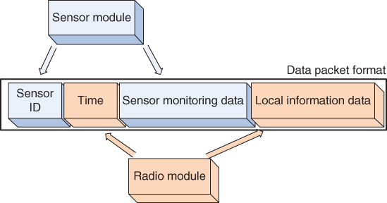
Figure 12.8 Data packet format.
12.4.3.2 Packet formation process
Every monitoring node forms packets and transmits data toward the destination. Packets are created every second, following the sampling rate of the sensor. The packet formation process is shown in Figure 12.8. Every packet has the following four fields:
- Sensor identifier: This identifier comes from the sensor module, and it is related with its product serial number. It is unique for every sensor module in the network. The identifier stores the number of the transmitter that sends the packet and allows the receiver to identify the origin of the packet. For every sensor ID there is a corresponding location stored at the control room. The location can be updated if the sensor is moved to a new location.
-
Time: The time comes from the radio module. This field stores the exact time when the packet was created. When a relay node receives the packets, it can place them in order based on the timestamps. For a
 monitoring application, the time is of high importance since it shows the variation of the
  levels over time.
 -
Sensor monitoring data: The data passed from the sensor to the radio module. The data field stores all the crucial information related with the
 concentration.
 - Local information data: This information comes from the radio module. This field includes information such as the remaining power level of a unit and average received signal strength indication (RSSI) for location information maintenance. RSSI can be used later on, when the traffic is low in the network, in order to update the location of the monitoring and relay nodes in the area.
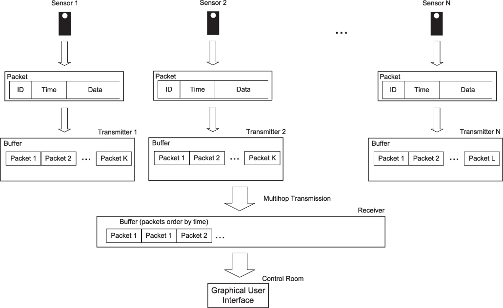
Figure 12.9 Packet process and transmission/reception.
12.4.3.3 Information Processing and Storage
The final information processing and storage takes place at the control room. Each packet is decomposed into different parts (sensor ID, time, data, etc.), and each part is plotted in real time. Further to real‐time processing, each part is stored into files to keep record of the data over time. The data is available to the system administrator off‐line for future reference.
The stored data is also used from the mobile node for calibration purposes. There are expected normal levels of ![]() in the different rooms of a building. This information is given to the mobile node to help with the calibration of the sensor units as well as with the initial configuration of newly deployed sensors. The information processing, transmission, and reception are shown in Figure 12.9.
in the different rooms of a building. This information is given to the mobile node to help with the calibration of the sensor units as well as with the initial configuration of newly deployed sensors. The information processing, transmission, and reception are shown in Figure 12.9.
12.4.4 Indoor Monitoring System
At the proposed monitoring system application, cognitive networking (Yucek and Arslan (2009), Liang et al. (2008)) is used along with opportunistic routing (Liu et al. (2009)) in a wireless multi‐hop network, for ![]() monitoring. An overview of the different system components is shown in Figure 12.10.
monitoring. An overview of the different system components is shown in Figure 12.10.
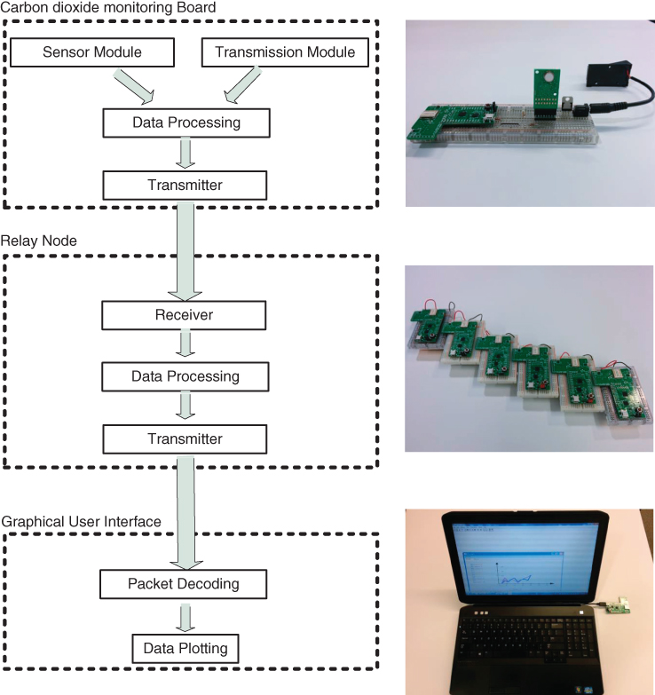
Figure 12.10 Overview of the monitoring system.
The final indoor monitoring board has two types of nodes: the wireless sensor nodes (monitoring boards) and the relay nodes. The wireless sensor nodes as well as the relay nodes are deployed in the building. The wireless sensor nodes know their relative location. The relay nodes will find their location during the initialization phase through the use of the RSSI. Each wireless sensor node is able to monitor the area around it, form packets, and forward these packets to one of the neighbor relay nodes, which will then forward the packet to the destination following the principles of the routing protocol.
12.5 Experiments and Results
In this section, the experimental setup is described, followed by a brief discussion of the results.

Figure 12.11
An indoor  detection and monitoring system deployed at the 7th floor of Bahen Centre for Information Technology at the University of Toronto. The sensor units have been deployed in four rooms: office ‐1, office ‐2, laboratory, and meeting room. The sensor units transmit the monitoring data to the control room through the relay nodes.
12.5.1 Experimental Setup
For the experiments of the proposed system, the 7th floor of Bahen Centre for Information Technology at the University of Toronto was used. A simplified floor map of the monitoring area is shown in Figure 12.11.
During the experiment, the ![]() concentration of four rooms was monitored: two offices, one laboratory, and one meeting room. The rooms were selected due to the different sizes and different number of occupants they can have during the day. Specifically:
concentration of four rooms was monitored: two offices, one laboratory, and one meeting room. The rooms were selected due to the different sizes and different number of occupants they can have during the day. Specifically:
- office ‐1, dimension
 , occupants (max) 3
 - office ‐2, dimension
 , occupants (max) 4
 - laboratory, dimension
 , occupants (max) 4
 - meeting room, dimension
 , occupants (max) 18
In all the monitoring rooms, the windows were closed during the experiment while the doors work with a mechanism that keeps them closed. The rooms are connected to the same central ventilation system. The system divides the rooms in clusters and controls the temperature of the different clusters in the floor.
Following the specifications of the rooms and the transmission range and the sensing range of the relay nodes and the sensor units, four sensor units were deployed, one in each room, and four relay nodes were placed outside each room. In the offices and the laboratory, the sensor units were placed at equal distances from the door and the workstation while in the meeting room the sensor unit was placed in the center of the room, hanging from the ceiling. The relay nodes follow a simple routing protocol that forwards the packets to the control room. The control room has a communication unit, similar to the relay nodes and sensing units, which collects all the data. The communication unit is attached to a laptop computer that processes the data, plots them in real time, and stores them in a database.
The experiments lasted for one month, between March 1 and March 31. The mobile node visited each monitoring room once per day for any necessary calibration. After the initial deployment, the system needed 15 minutes to reach a stable level. Both the relay nodes and the sensor unit were moved throughout the experimental period, and the new positions were found with the use of the RSSI value. There was no hardware failure during the experimentation while some of the nodes needed battery replacement.

Figure 12.12
Time series representation of air quality measurements at office ‐ 2 over  hours before and after smoothing.
12.5.2 Results Analysis
Initially, the information processing unit was evaluated. During the experiments, some of the data were corrupted or not accurate. Outliers needed to be detected and removed to improve system reliability.
The sensor data before and after the proposed data smoothing algorithm in office‐ 2 and for 12 hours is shown in Figure 12.12. The sensor unit in office‐ 2 stored all the sensor data during the experiments. These data are compared with the data the sensor transmits toward the control room, after the processing. It is clear that periodic outliers for a few seconds are cleared and ignored from the system. The decision for the potential outlier is taken at the sensor unit and is based on the outlier window of 10 sec as described in the previous section.
Similarly, the sensor data before and after smoothing in the meeting room and for a months is shown in Figure 12.13. The smoothing this time takes place at the control room. The algorithm examines the reported data in an hour period and decides the value. In a month period, the smoothing algorithm is necessary to remove noise from the data that was not removed locally inside each monitoring node.

Figure 12.13 Time series representation of air quality measurements at meeting room over March 2015 before and after smoothing.
The concentration of ![]() for 12 hours, from the morning to the afternoon, is shown in Figure 12.14. The measurements are during the peak hours at the examined rooms. Several people are moving between the rooms, working on computers, and opening and closing the doors. Both people and computers contribute to the
for 12 hours, from the morning to the afternoon, is shown in Figure 12.14. The measurements are during the peak hours at the examined rooms. Several people are moving between the rooms, working on computers, and opening and closing the doors. Both people and computers contribute to the ![]() levels. It is expected that when the number of people in the room increases, the
levels. It is expected that when the number of people in the room increases, the ![]() concentration increases as well.
concentration increases as well.
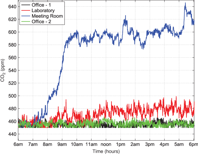
Figure 12.14
Time series representation of air quality measurements over  hours.
In the early morning, between ![]() and
and ![]() all the rooms report similar
all the rooms report similar ![]() levels. This is expected, since the rooms are empty. Also, there is not great variation between the different room sizes since the size should not affect the
levels. This is expected, since the rooms are empty. Also, there is not great variation between the different room sizes since the size should not affect the ![]() levels.
levels.
As people start coming into the examined area, there are some noticeable differences. The concentration in the two offices increases; however, because the number of the people is low, the increase is small. In the laboratory, the increase is higher than in the offices. This is due to the higher number of people who visit the laboratory during the day. It is also interesting to notice that when the conditions are normal (no fire detection, etc.), based on the reported levels of ![]() , it can be inferred that the number of people in the laboratory is higher than the number of the people in the offices.
, it can be inferred that the number of people in the laboratory is higher than the number of the people in the offices.
The greatest increase is shown in the meeting room. As the number of people in the meeting room increases, ![]() concentration reported increases from around
concentration reported increases from around ![]() to
to ![]() . The introduced system managed to report an increase in the level that is related to the people's presence and activity in the room (Fonollosa et al. (2014)).
. The introduced system managed to report an increase in the level that is related to the people's presence and activity in the room (Fonollosa et al. (2014)).

Figure 12.15 Time series representation of air quality measurements over March 2015.
Finally, the concentration for the four rooms over a month is shown in Figure 12.15. As it can be inferred, the days the monitoring rooms have a high number of people is clearly noticeable. Especially in the meeting room, when it is used, the concentration is clearly higher than the normal levels. Similarly for the laboratory, based on students activities, some days throughout the month the levels are high. The concentration of ![]() in the offices seems stable and around normal during the monitoring month.
in the offices seems stable and around normal during the monitoring month.
12.6 Conclusions
In this chapter, an environmental‐monitoring system for smart buildings was proposed. The drawbacks of traditional methods for monitoring were discussed, followed by a review of some commonly used WSN‐monitoring applications. Then, the requirements and challenges along with the design goal of the proposed system were discussed.
A framework was proposed, implemented, and examined for real‐time environmental monitoring in a building. The necessary design decisions, hardware components, and information processing units were presented.
In the last part, experimental results over a month period from the introduced testbed were shown. A useful insight from the result is that data filtering and smoothing can help to improve the reliability of the system. Also, as it can be inferred from the results, the number of the occupants in the room affects the environmental quality in the room. In future studies, this could also be used as an estimation for the number of people in a room.
Environmental monitoring is a crucial task for smart buildings. WSNs is a promising solution due to the many advantages and the minimum energy requirements.
References
- I. F. Akyildiz, Weilian Su, Y. Sankarasubramaniam, and E. Cayirci. A survey on sensor networks. IEEE Communications Magazine, 40(8):102–114, Aug. 2002. ISSN 0163‐6804. doi: 10.1109/MCOM.2002.1024422.
- J. N. Al‐Karaki and A. E. Kamal. Routing techniques in wireless sensor networks: a survey. IEEE Wireless Communications, 11(6):6–28, Dec. 2004. ISSN 1536‐1284. doi: 10.1109/MWC.2004.1368893.
- T. Arampatzis, J. Lygeros, and S. Manesis. A survey of applications of wireless sensors and wireless sensor networks. In Proceedings of the 2005 IEEE International Symposium on, Mediterrean Conference on Control and Automation Intelligent Control, 2005., pages 719–724, June 2005. doi: 10.1109/.2005.1467103.
- P. Bellavista, G. Cardone, A. Corradi, and L. Foschini. Convergence of manet and wsn in iot urban scenarios. IEEE Sensors Journal, 13(10):3558–3567, Oct 2013a. ISSN 1530‐437X. doi: 10.1109/JSEN.2013.2272099.
- P. Bellavista, G. Cardone, A. Corradi, and L. Foschini. Convergence of manet and wsn in iot urban scenarios. IEEE Sensors Journal, 13(10):3558–3567, Oct. 2013b. ISSN 1530‐437X. doi: 10.1109/JSEN.2013.2272099.
- L. Bencini, F. Chiti, G. Collodi, D. D. Palma, R. Fantacci, A. Manes, and G. Manes. Agricultural monitoring based on wireless sensor network technology: Real long life deployments for physiology and pathogens control. In 2009 Third International Conference on Sensor Technologies and Applications, pages 372–377, June 2009. doi: 10.1109/SENSORCOMM.2009.63.
- A. Boubrima, W. Bechkit, and H. Rivano. Optimal wsn deployment models for air pollution monitoring. IEEE Transactions on Wireless Communications, 16(5):2723–2735, May 2017. ISSN 1536‐1276. doi: 10.1109/TWC.2017.2658601.
- G. Cardone, L. Foschini, P. Bellavista, A. Corradi, C. Borcea, M. Talasila, and R. Curtmola. Fostering participaction in smart cities: a geo‐social crowdsensing platform. IEEE Communications Magazine, 51(6):112–119, June 2013. ISSN 0163‐6804. doi: 10.1109/MCOM.2013.6525603.
- CCOHS. Canadian Centre for Occupational Health and Safety. Indoor Air Quality, Jul. 2013.
- A. Chirap, V. Popa, E. Coca, and D. A. Potorac. A study on light energy harvesting from indoor environment: The autonomous sensor nodes. In 2014 International Conference on Development and Application Systems (DAS), pages 127–131, May 2014. doi: 10.1109/DAAS.2014.6842441.
- CO2Meter. iAQ‐2000 Indoor Air Quality (VOC) Sensor. http://www.co2meter.com/products/iaq‐2000‐indoor‐air‐quality‐sensor.
- P. Corral, J. A. Perez, A. C. De Castro Lima, and O. Ludwig. Parking spaces detection in indoor environments based on zigbee. IEEE Latin America Transactions, 10(1):1162–1167, Jan. 2012. ISSN 1548‐0992. doi: 10.1109/TLA.2012.6142454.
- EPA. Buildings and their Impact on the Environment: A statistical Summary. U.S. Environmental Protection Agency Green Building Workgroup, Oct. 2014.
- S. Fang, L. D. Xu, Y. Zhu, J. Ahati, H. Pei, J. Yan, and Z. Liu. An integrated system for regional environmental monitoring and management based on internet of things. IEEE Transactions on Industrial Informatics, 10(2):1596–1605, May 2014. ISSN 1551‐3203. doi: 10.1109/TII.2014.2302638.
- J. Fonollosa, I. Rodriguez‐Lujan, A. V. Shevade, M. L. Homer, M. A. Ryan, and R. Huerta. Human activity monitoring using gas sensor arrays. Sensors and Actuators B: Chemical, 199:398–402, Aug. 2014.
- D.S. Ghataoura, J.E. Mitchell, and G.E. Matich. Networking and application interface technology for wireless sensor network surveillance and monitoring. Communications Magazine, IEEE, 49(10):90–97, Oct. 2011. ISSN 0163‐6804. doi: 10.1109/MCOM.2011.6035821.
- Z. Guo, Y. Guo, F. Hong, Z. Jin, Y. He, Y. Feng, and Y. Liu. Perpendicular intersection: Locating wireless sensors with mobile beacon. IEEE Transactions on Vehicular Technology, 59(7):3501–3509, Sept. 2010. ISSN 0018‐9545. doi: 10.1109/TVT.2010.2049391.
- B. N. Hood and P. Barooah. Estimating doa from radio‐frequency rssi measurements using an actuated reflector. IEEE Sensors Journal, 11(2): 413–417, Feb. 2011. ISSN 1530‐437X. doi: 10.1109/JSEN.2010.2070872.
- M. Fahim Jan, Q. Habib, M. Irfan, M. Murad, K. M. Yahya, and G. M. Hassan. Carbon monoxide detection and autonomous countermeasure system for a steel mill using wireless sensor and actuator network. In 2010 6th International Conference on Emerging Technologies (ICET), pages 405–409, Oct. 2010. doi: 10.1109/ICET.2010.5638502.
- V. Jelicic, M. Magno, D. Brunelli, G. Paci, and L. Benini. Context‐Adaptive Multimodal Wireless Sensor Network for Energy‐Efficient Gas Monitoring. Sensors Journal, IEEE, 13(1):328–338, Jan. 2013. ISSN 1530‐437X. doi: 10.1109/JSEN.2012.2215733.
- J. Jin, J. Gubbi, S. Marusic, and M. Palaniswami. An information framework for creating a smart city through internet of things. IEEE Internet of Things Journal, 1(2):112–121, April 2014a. ISSN 2327‐4662. doi: 10.1109/JIOT.2013.2296516.
- J. Jin, J. Gubbi, S. Marusic, and M. Palaniswami. An information framework for creating a smart city through internet of things. IEEE Internet of Things Journal, 1(2):112–121, April 2014b. ISSN 2327‐4662. doi: 10.1109/JIOT.2013.2296516.
- R. Kays, S. Tilak, M. Crofoot, T. Fountain, D. Obando, A. Ortega, F. Kuemmeth, J. Mandel, G. Swenson, T. Lambert, B. Hirsch, and M. Wikelski. Tracking animal location and activity with an automated radio telemetry system in a tropical rainforest. The Computer Journal, 54(12):1931, 2011. doi: 10.1093/comjnl/bxr072. URL +http://dx.doi.org/10.1093/comjnl/bxr072.
- S.D.T. Kelly, N.K. Suryadevara, and S.C. Mukhopadhyay. Towards the Implementation of IoT for Environmental Condition Monitoring in Homes. Sensors Journal, IEEE, 13(10):3846–3853, Oct. 2013. ISSN 1530‐437X. doi: 10.1109/JSEN.2013.2263379.
- J. Kim, C. Chu, and S. Shin. ISSAQ: An Integrated Sensing Systems for Real‐Time Indoor Air Quality Monitoring. Sensors Journal, IEEE, 14(12): 4230–4244, Dec. 2014. ISSN 1530‐437X.
- N. Lathia, V. Pejovic, K. K. Rachuri, C. Mascolo, M. Musolesi, and P. J. Rentfrow. Smartphones for large‐scale behavior change interventions. IEEE Pervasive Computing, 12(3):66–73, July 2013. ISSN 1536‐1268. doi: 10.1109/MPRV.2013.56.
- Y. C. Liang, Y. Zeng, E. C. Y. Peh, and A. T. Hoang. Sensing‐throughput tradeoff for cognitive radio networks. IEEE Transactions on Wireless Communications, 7(4):1326–1337, April 2008. ISSN 1536‐1276. doi: 10.1109/TWC.2008.060869.
- H. Liu, B. Zhang, H. T. Mouftah, X. Shen, and J. Ma. Opportunistic routing for wireless ad hoc and sensor networks: Present and future directions. IEEE Communications Magazine, 47(12):103–109, Dec 2009. ISSN 0163‐6804. doi: 10.1109/MCOM.2009.5350376.
- C. Maihofer. A survey of geocast routing protocols. IEEE Communications Surveys Tutorials, 6(2):32–42, Second 2004. ISSN 1553‐877X. doi: 10.1109/COMST.2004.5342238.
- A. Mainwaring, D. Culler, J. Polastre, R. Szewczyk, and J. Anderson. Wireless sensor networks for habitat monitoring. In Proceedings of the 1st ACM International Workshop on Wireless Sensor Networks and Applications, WSNA '02, pages 88–97, New York, NY, USA, 2002. ACM. ISBN 1‐58113‐589‐0. doi: 10.1145/570738.570751. URL http://doi.acm.org/10.1145/570738.570751.
- X. Mao, X. Miao, Y. He, X. Li, and Y. Liu. CitySee: Urban CO2 monitoring with sensors. In INFOCOM, 2012 Proceedings IEEE, pages 1611–1619, Mar. 2012. doi: 10.1109/INFCOM.2012.6195530.
- I. Martin, T. O'Farrell, R. Aspey, S. Edwards, T. James, P. Loskot, T. Murray, I. Rutt, N. Selmes, and T. Baugé. A high‐resolution sensor network for monitoring glacier dynamics. IEEE Sensors Journal, 14(11):3926–3931, Nov. 2014. ISSN 1530‐437X. doi: 10.1109/JSEN.2014.2348534.
- L. Oliveira and J. Rodrigues. Wireless sensor networks: a survey on environmental monitoring. Journal of Communications, Special Issue: Recent Advance on Distributed Sensor Systems and Applications, 6(2):143 –151, 2011.
- OMESH Networks. OPM15. http://www.omeshnet.com/omesh/.
- M. Othman and K. Shazali. Wireless sensor network applications: A study in environment monitoring system. Procedia Engineering, 41:1204 –1210, 2012. ISSN 1877‐7058. doi: http://dx.doi.org/10.1016/j.proeng.2012.07.302. URL http://www.sciencedirect.com/science/article/pii/S1877705812027026.
- N. A. Pantazis, S. A. Nikolidakis, and D. D. Vergados. Energy‐efficient routing protocols in wireless sensor networks: A survey. IEEE Communications Surveys Tutorials, 15(2):551–591, Second 2013. ISSN 1553‐877X. doi: 10.1109/SURV.2012.062612.00084.
- C. Peng, K. Qian, and C. Wang. Design and Application of a VOC‐Monitoring System Based on a ZigBee Wireless Sensor Network. Sensors Journal, IEEE, 15(4): 2255–2268, Apr. 2015. ISSN 1530‐437X. doi: 10.1109/JSEN.2014.2374156.
- O.A. Postolache, J.M.D. Pereira, and P.M.B.S. Girao. Smart sensors network for air quality monitoring applications. Instrumentation and Measurement, IEEE Transactions on, 58(9):3253–3262, Sept 2009. ISSN 0018‐9456. doi: 10.1109/TIM.2009.2022372.
- E. Sazonov, Haodong Li, D. Curry, and P. Pillay. Self‐Powered Sensors for Monitoring of Highway Bridges. Sensors Journal, IEEE, 9(11):1422–1429, Nov. 2009. ISSN 1530‐437X. doi: 10.1109/JSEN.2009.2019333.
- X. Sheng, J. Tang, X. Xiao, and G. Xue. Sensing as a service: Challenges, solutions and future directions. IEEE Sensors Journal, 13(10):3733–3741, Oct. 2013. ISSN 1530‐437X. doi: 10.1109/JSEN.2013.2262677.
- H. Shin, Y. Chon, and H. Cha. Unsupervised construction of an indoor floor plan using a smartphone. IEEE Transactions on Systems, Man, and Cybernetics, Part C (Applications and Reviews), 42(6):889–898, Nov. 2012. ISSN 1094‐6977. doi: 10.1109/TSMCC.2011.2169403.
- P. Spachos and D. Hantzinakos. Scalable Dynamic Routing Protocol for Cognitive Radio Sensor Networks. Sensors Journal, IEEE, 14(7):2257–2266, Jul. 2014. ISSN 1530‐437X. doi: 10.1109/JSEN.2014.2309138.
- P. Spachos and D. Hatzinakos. Poster: Cognitive networking in a self‐powered wireless sensor network testbed. In Proceedings of the 20th Annual International Conference on Mobile Computing and Networking, MobiCom '14, pages 425–428, New York, NY, USA, 2014. ACM. ISBN 978‐1‐4503‐2783‐1. doi: 10.1145/2639108.2642909. URL http://doi.acm.org/10.1145/2639108.2642909.
- P. Spachos and D. Hatzinakos. Self‐powered wireless sensor network for environmental monitoring. In 2015 IEEE Globecom Workshops (GC Wkshps), pages 1–6, Dec. 2015. doi: 10.1109/GLOCOMW.2015.7414207.
- P. Spachos and D. Hatzinakos. Real‐time indoor carbon dioxide monitoring through cognitive wireless sensor networks. IEEE Sensors Journal, 16(2): 506–514, Jan. 2016. ISSN 1530‐437X. doi: 10.1109/JSEN.2015.2479647.
- P. Spachos, F. M. Bui, Liang Song, Y. Lostanlen, and D. Hatzinakos. Performance evaluation of wireless multihop communications for an indoor environment. In 2011 IEEE 22nd International Symposium on Personal, Indoor and Mobile Radio Communications, pages 1140–1144, Sept. 2011. doi: 10.1109/PIMRC.2011.6139676.
- P. Spachos, P. Chatzimisios, and D. Hatzinakos. Energy aware opportunistic routing in wireless sensor networks. In Globecom Workshops (GC Wkshps), 2012 IEEE, pages 405–409, Dec 2012. doi: 10.1109/GLOCOMW.2012.6477606.
- P. Spachos, J. Lin, H. Bannazadeh, and A. Leon‐Garcia. Smart room monitoring through wireless sensor networks in software defined infrastructures. In Cloud Networking (CloudNet), 2015 IEEE 4th International Conference on, pages 216–218, Oct 2015. doi: 10.1109/CloudNet.2015.7335310.
- E. Suganya and S. Vijayashaarathi. Smart vehicle monitoring system for air pollution detection using wsn. In 2016 International Conference on Communication and Signal Processing (ICCSP), pages 0719–0722, April 2016. doi: 10.1109/ICCSP.2016.7754238.
- T. Torfs, T. Sterken, S. Brebels, J. Santana, R. van den Hoven, V. Spiering, N. Bertsch, D. Trapani, and D. Zonta. Low Power Wireless Sensor Network for Building Monitoring. Sensors Journal, IEEE, 13(3):909–915, Mar. 2013. ISSN 1530‐437X. doi: 10.1109/JSEN.2012.2218680.
- W. Tsujita, H. Ishida, and T. Moriizumi. Dynamic gas sensor network for air pollution monitoring and its auto‐calibration. In Sensors, 2004. Proceedings of IEEE, pages 56–59 vol.1, Oct. 2004. doi: 10.1109/ICSENS.2004.1426098.
- H. Yang, Y. Qin, G. Feng, and H. Ci. Online Monitoring of Geological Storage and Leakage Based on Wireless Sensor Networks. Sensors Journal, IEEE, 13(2):556–562, Feb. 2013. ISSN 1530‐437X. doi: 10.1109/JSEN.2012.2223210.
- J. Yick, B. Mukherjee, and D. Ghosal. Wireless sensor network survey. Computer Networks, 52(12):2292–2330, 2008. ISSN 1389‐1286. doi: https://doi.org/10.1016/j.comnet.2008.04.002. URL http://www.sciencedirect.com/science/article/pii/S1389128608001254.
- H. Yu and Q. Yue. Indoor light energy harvesting system for energy‐aware wireless sensor node. Energy Procedia, 16:1027–1032, 2012. ISSN 1876‐6102. doi: http://dx.doi.org/10.1016/j.egypro.2012.01.164. URL http://www.sciencedirect.com/science/article/pii/S1876610212001749.
- T. Yucek and H. Arslan. A survey of spectrum sensing algorithms for cognitive radio applications. IEEE Communications Surveys Tutorials, 11(1):116–130, First 2009. ISSN 1553‐877X. doi: 10.1109/SURV.2009.090109.
- A. Zanella, N. Bui, A. Castellani, L. Vangelista, and M. Zorzi. Internet of things for smart cities. IEEE Internet of Things Journal, 1(1):22–32, Feb. 2014. ISSN 2327‐4662. doi: 10.1109/JIOT.2014.2306328.
- M. Zorzi and R. R. Rao. Geographic random forwarding (geraf) for ad hoc and sensor networks: multihop performance. IEEE Transactions on Mobile Computing, 2(4):337–348, Oct. 2003. ISSN 1536‐1233. doi: 10.1109/TMC.2003.1255648.