23
Spatiotemporal Big Data Analysis for Smart Grids Based on Random Matrix Theory
Robert Qiu1,2,3 Lei Chu2,3 Xing He2,3 Zenan Ling2,3 and Haichun Liu2,3
1 Tennessee Technological University, Cookeville, TN, 38505, USA
2 Department of Electrical Engineering, Shanghai Jiaotong University, Shanghai, 200240, China
3 Research Center for Big Data Engineering and Technology, State Energy Smart Grid Research and Development Center, Shanghai, China
A cornerstone of the smart grid is the advanced monitorability on its assets and operations. Increasingly pervasive installation of phasor measurement units (PMUs) allows the so‐called synchrophasor measurements to be taken roughly 100 times faster than the legacy supervisory control and data acquisition (SCADA) measurements, time‐stamped using the Global Positioning System (GPS) signals to capture the grid dynamics. On the other hand, the availability of low‐latency two‐way communication networks will pave the way to high‐precision real‐time grid state estimation and detection, remedial actions upon network instability, and accurate risk analysis and post‐event assessment for failure prevention.
In this chapter, we firstly model spatiotemporal PMU data in large‐scale grids as random matrix sequences. Secondly, some basic principles of random matrix theory (RMT), such as asymptotic spectrum laws, transforms, convergence rate, and free probability, are introduced briefly in order to improve the understanding and application of RMT technologies. Lastly, the case studies based on synthetic data and real data are developed to evaluate the performance of the RMT‐based schemes in different application scenarios (i.e., state evaluation and situation awareness).
23.1 Introduction
23.1.1 Perspective on Smart Grids
The modern power grid is one of the most complex engineering systems in existence; the North American power grid is recognized as the supreme engineering achievement in the 20th century [1]. The complexity of the future's electrical grid is ever increasing: (1) the evolution of the grid network, especially the expansion in size; (2) the penetration of renewable/distributed resources, flexible/controllable electronic units, or even prosumers with dual load‐generator behavior [2]; and (3) the revolution of the operation mechanism, e.g., demand‐side management. Also, financial, environmental, and regulatory constraints are pushing the electrical grid toward its stability limit.
Generally, power grids have experienced three ages—G1, G2, and G3 [3]. The network structures are depicted in Figure 23.1 [4]. Their data flows and energy flows, as well as corresponding data management systems and work modes, are quite different [5], which are shown in Figure 23.2 and Figure 23.3, respectively.
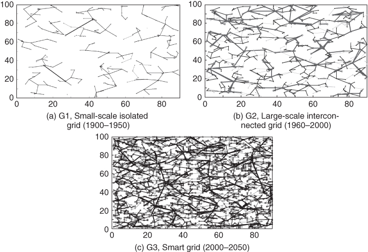
Figure 23.1 Topologies of Grid Network.

Figure 23.2 Data flows and energy flows for three generations of power systems. The single lines, double lines, and triple lines indicate the flows of G1, G2, and G3, respectively.

Figure 23.3 Data management systems and work modes for three ages of power systems. The above, middle, and below parts indicate the data management systems and the work modes of G1, G2, and G3, respectively. For G1, each grid works independently. For G2, global and local control centers are operating under the team‐work mode. For G3, the group‐work mode breaks through the regional limitation for energy.
![]()
G1 was developed from the power system around 1900 to 1950, featured by small‐scale isolated grids. For G1, units interchange energy and data within the isolated grid to keep generation‐consumption balance. The units are mostly controlled by themselves, i.e., operating under individual‐work mode. As shown in Figure 23.1(a), each apparatus collects designated data and makes corresponding decisions only with its own application. The individual‐work mode works with an easy logic and little information communication. However, it means few advanced functions and inefficient utilization of resources. It is only suitable for small grids or isolated islands.
![]()
G2 was developed from power grids about 1960 to 2000, featured by zone‐dividing large‐scale interconnected grids. For G2, units interchange energy and data with adjacent units. The units are dispatched by a control center, i.e., they are operating under team‐work mode. The regional team leaders, such as local dispatching centers, substations, and microgrid control centers, aggregate their own team members (i.e., units in the region) into a standard black‐box model. These standard models will be further aggregated by the global control center for control or prediction purposes. The two aggregations above are achieved by four steps: data monitoring, data preprocessing, data storage, and data processing. The description above can be summarized by by dotted blue lines in Figure 23.3. In general, the team‐work mode conducts model‐based analysis and mainly concerns system stability rather than individual benefit; it does not work well for smart grids with 4Vs data.
![]()
The development of G3 was launched at the beginning of the 21st century, and for China, it is expected to be completed around 2050 [ 3]. Figure 23.1(c) shows that the clear‐cut partitioning is no longer suitable for G3, as well as the team‐work mode, which is based on the regional leader. For G3, the individual units, rather than the regional center (if it still exists), play a dominant role. They are appropriately self‐controlled with high intelligence, resulting in much more flexible flows for both energy exchange and data communication [6]. Accordingly, the group‐work mode is proposed. Under this mode, the individuals freely operate under the supervision of the global control centers [ 5]. VPPs [7], MMGs [8], for instance, are typically G3 utilities. These group‐work mode utilities provide a relaxed environment to benefit both individuals and the grids: the former, driven by their own interests and characteristics, are able to create or join a relatively free group to benefit mutually from sharing their own superior resources; meanwhile, these utilities are often big and controllable enough to be good customers or managers to the grids.
23.1.2 The Role of Data in the Future Power Grid
Data are more and more easily accessible in smart grids. Figure 23.4 shows numerous data sources: information communication technology (ICT), advanced metering infrastructure (AMI), supervisory control and data acquisition (SCADA), sensor technology (ST), phasor measurement units (PMUs), and intelligent electronic devices (IEDs) [9]. Hence, data with features of volume, velocity, variety, and veracity (i.e., 4Vs data) [10] are inevitably generated and daily aggregated. Particularly, the “4Vs” are elaborated as follows:
- Volume. There are massive data in power grids. The so‐called curse of dimensionality [11] occurs inevitably. The worldwide small‐scale roof‐top photovoltaics (PVs) installation reached 23 GW at the end of 2013, and the growth is predicted to be 20 GW per year until 2018. The uptake of electric vehicles (EVs) also continues to grow. At least 665,000 electric‐drive light‐duty vehicles, 46,000 electric buses, and 235 million electric two‐wheelers were in the worldwide market in early 2015 [12].
- Velocity. The resource costs (time, hardware, human, etc.) for big data analytics should be tolerable. To sever online decision making, massive data must be processed within a fraction of second.
- Variety. The data in various formats are often derived from diverse departments. In the view of data management, sampling frequency of source data, processing speed, and service objects are not completely accord.
- Veracity. For a massive data source, there often exist realistic bad data, e.g., incomplete, inaccurate, asynchronous, and unavailable. For system operations, decisions such as protection should be highly reliable.

Figure 23.4 Smart grid with 4Vs data and its SA.
As mentioned above, smart grids are always huge in size and complex in topology; big data analytics and a data‐driven approach become natural solutions for the future grid [13–16]. Driven by data analysis in high dimension, big data technology works out data correlations (indicated by statistical parameters) to gain insight to the inherent mechanisms. Actually, big data technology has already been successfully applied as a powerful data‐driven tool for numerous phenomena, such as quantum systems [17], financial systems [18, 19], biological systems [20], as well as wireless communication networks [21–23]. For smart grids, the data‐driven approach and data utilization are currently important topics, as evidenced in the special issue of “Big Data Analytics for Grid Modernization” [24]. This special issue is most relevant to our book in spirit. Several SA topics are discussed as well. We highlight anomaly detection and classification [25, 26], social media such as Twitter in [27], the estimation of active ingredients such as PV installations [28, 29], and finally the real‐time data for online transient stability evaluation [30]. In addition, we point out research about the improvement in wide‐area monitoring, protection and control (WAMPAC) and the utilization of PMU data [31–34], together with the fault detection and location [35–37]. Xie et al., based on principal component analysis (PCA), proposes an online application for early event detection by introducing a reduced dimensionality [38]. Lim et al. studies the quasi‐steady‐state operational problems relevant to the voltage instability phenomena [39]. These works provide primary exploration of the big data analysis in the smart grid. Furthermore, a brief account for random matrix theory (RMT), which can be seen as basic analysis tools for spatial‐temporal grid data processing, is elaborated in the following subsection.
23.1.3 A Brief Account for RMT
The last two decades have seen the rapid growth of RMT in many science fields. Brilliant mathematical work in RMT shed light on the challenges of classical statistics. In this subsection, we present a brief introduction to the main development of RMT. The application‐related account, with particular attention paid to recently rising RMT‐based technology that are relevant for the smart grid, is elaborated in Section 23.3.
The research of random matrices began with the work of Wishart in 1928, which focused on the distribution of the sample covariance matrices. The first asymptotic results on the limit spectrum of large random matrices (energy levels of nuclei) were obtained by Wigner in 1950s in a series of works [40–43] which ultimately lead to the well‐known semicircle law [44]. Another breakthrough was presented in [45], which studied the distribution of eigenvalues for empirical covariance matrices. Based on these excellent works, RMT became a vibrant research direction of its own. Plenty of brilliant works that branched off the early physical and statistical applications were put forward in the last decades. For the sake of brevity, here we only show two remarkable results that turned out to be related to a large number of research hotspots in economics, communications, and the smart grid. One of the most striking advances is the discovery of the Tracy Widom distribution of extreme eigenvalues and another one is the single ring law, which described the limit spectrum of eigenvalues of non‐normal square matrices [46]. Interested readers are referred to monographs [47–49] for more details.
We will end this section by providing the structure of the remainder of this chapter.
Firstly, Section 23.2 gives a tutorial account of existing mathematical works that are relevant to the statistical analysis of random matrices arising in smart grids. Specially, Section 23.2.1 introduces data collected from the widely applied phasor measurement unit and data modeling using linear and nonlinear combinations of random matrices. Section 23.2.2 focuses on asymptotic spectrum laws of the major types of random matrices. Section 23.2.3 presents three dominant transforms that play key roles in describing the limit spectra of random matrices. Recent results on the convergence rate to the asymptotic limits are contained in Section 23.2.4. Section 23.2.5 is dedicated to free probability theory, which is demonstrated as a practical tool for smart grids.
Secondly, we begin with some representative problems arisen from the wide deployment of synchronous phasor measurement units that capture various features of interest in smart grids. We then show how random matrix theory has been used to characterize the data collected from synchronous phasor measurement and tackle the problems in the era of big data. In particular, Section 23.3.1 provides some basis hypothesis tests that remain fundamental to research into the behavior of the data in smart grids. Section 23.3.2 concerns stability assessment from some recently developed data‐driven methods based on RMT. Section 23.3.3 focuses on situation awareness for smart grids from linear eigenvalue statistics. The early event detection problem is studied in detail using free probability in Section 23.3.4.
23.2 RMT: A Practical and Powerful Big Data Analysis Tool
In this section, we provide comprehensive existing mathematical results that are associated with the analysis of statistics of random matrices arising in smart grids. We also describe some new results on random matrices and other data‐driven methods that were inspired by problems of engineering interest.
23.2.1 Modeling Grid Data using Large Dimensional Random Matrices
Before the comprehensive utilization of the RMT framework, we try to build a model for spatiotemporal PMU data using large dimensional random matrices.
It is well accepted that the transient behavior of a large electric power system can be illustrated by a set of differential and algebraic equations (DAEs) as follows [50]:
where ![]() are the power state variables, e.g., rotor speeds and the dynamic states of loads,
are the power state variables, e.g., rotor speeds and the dynamic states of loads, ![]() represent the system input parameters,
represent the system input parameters, ![]() define algebraic variables, e.g., bus voltage magnitudes,
define algebraic variables, e.g., bus voltage magnitudes, ![]() denote the time‐invariant system parameters.
denote the time‐invariant system parameters. ![]() ,
, ![]() and
and ![]() are the sample time, number of system variables, and bus, respectively. The model‐based stability estimators [51, 52] focus on linearization of nonlinear DAEs in (23.1) and (23.2) which gives
are the sample time, number of system variables, and bus, respectively. The model‐based stability estimators [51, 52] focus on linearization of nonlinear DAEs in (23.1) and (23.2) which gives

where ![]() ,
, ![]() are the Jacobian matrices of
are the Jacobian matrices of ![]() with respect to
with respect to ![]() and
and ![]() .
. ![]() is a diagonal matrix whose diagonal entries equal
is a diagonal matrix whose diagonal entries equal ![]() and
and ![]() is the correction time of the load fluctuations.
is the correction time of the load fluctuations. ![]() denotes a diagonal matrix whose diagonal entries are nominal values of the corresponding active
denotes a diagonal matrix whose diagonal entries are nominal values of the corresponding active ![]() or reactive
or reactive ![]() of loads;
of loads; ![]() is assumed to be a vector of independent Gaussian random variables.
is assumed to be a vector of independent Gaussian random variables.
It is noted that estimating the system stability by solving the equation (23.3) is becoming increasingly more challenging [ 49] as a consequence of the steady growth of the parameters, say, ![]() ,
, ![]() , and
, and ![]() . Besides, the assumption that
. Besides, the assumption that ![]() follows a Gaussian distribution would restrict the practical applications.
follows a Gaussian distribution would restrict the practical applications.
On the other hand, as a novel alternative, the lately advanced data‐driven estimators [38, 39, 52, 53] can assess stability without knowledge of the power network parameters or topology. However, these estimators are based on the analysis of individual window‐truncated PMU data. In this chapter, we seek to provide a method with the ability of continuous learning of power system for spatiotemporal PMU data.
Firstly, we provide a novel method for modeling spatiotemporal PMU data. Figure 23.5 illustrates the conceptual representation of the structure of the spatiotemporal PMU data. More specifically, let ![]() denote the number of the available PMUs across the whole power network, each providing
denote the number of the available PMUs across the whole power network, each providing ![]() measurements. At the
measurements. At the ![]() th time sample, a total of
th time sample, a total of ![]() measurements, say
measurements, say ![]() , are collected. With respect to each PMU, the
, are collected. With respect to each PMU, the ![]() measurements could contain many categories of variables, such as voltage magnitude, power flow and frequency, etc. In this chapter, we develop PMU data analysis assuming each type of measurements is independent. That is, we assume that at each round of analysis,
measurements could contain many categories of variables, such as voltage magnitude, power flow and frequency, etc. In this chapter, we develop PMU data analysis assuming each type of measurements is independent. That is, we assume that at each round of analysis, ![]() . Given
. Given ![]() time periods of
time periods of ![]() seconds with
seconds with ![]() Hz sampling frequency in the
Hz sampling frequency in the ![]() th data collection. Let
th data collection. Let ![]() and
and ![]() , a sequence of large random matrix
, a sequence of large random matrix

is obtained to represent the collected voltage PMU measurements.
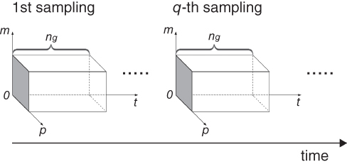
Figure 23.5 Conceptual representation of the structure of the spatiotemporal PMU data.
As illustrated in Figure 23.5, ![]() is a large random matrix with independent identical distributed entries. Here we also include other forms of basic random matrices that are relevant to the applications in smart grids as follows.
is a large random matrix with independent identical distributed entries. Here we also include other forms of basic random matrices that are relevant to the applications in smart grids as follows.
Gaussian unitary ensemble (GUE): Let ![]() be
be ![]() Wigner matrix, also known as Gaussian unitary ensemble GUE, and
Wigner matrix, also known as Gaussian unitary ensemble GUE, and ![]() .
. ![]() satisfies the following conditions:
satisfies the following conditions:
- The entries of
 are
are  Gaussian variables.
 - For
 ,
,  and
and  are
are  with distribution
  .
. - For any
 in
in  ,
,  .
. - The diagonal entries of
 are real random variables with distribution
  .
.
For the convenience of analysis, we can denote GUE as ![]() . Besides, the joint
. Besides, the joint ![]() of ordered eigenvalues of GUE
of ordered eigenvalues of GUE ![]() is [54, 55]
is [54, 55]

Laguerre unitary ensemble (LUE): Let ![]() be
be ![]() Gaussian random variables with
Gaussian random variables with ![]() and
and ![]() . The so called Wishart matrix or Laguerre unitary ensemble LUE can be expressed as
. The so called Wishart matrix or Laguerre unitary ensemble LUE can be expressed as ![]() . The
. The ![]() of
of ![]() for
for ![]() is [47, 55]
is [47, 55]

Large random matrix polynomials:
where ![]() are analytical functions,
are analytical functions, ![]() is a GUE, and
is a GUE, and ![]() is a LUE. See more details in Section 23.2.5.
is a LUE. See more details in Section 23.2.5.
23.2.2 Asymptotic Spectrum Laws
In this subsection, we provide a brief introduction to the asymptotic spectrum laws of the large basic random matrices, as shown in Section 23.2.1. There are remarkable results describing the asymptotic spectrum laws. Here special attention is paid to the limit behavior of marginal eigenvalues as the data dimensions tend to infinity.
We start with the GUE matrix ![]() whose entries are independent identical distributed zero‐mean (real or complex) Gaussian ensembles. As shown in [47], as
whose entries are independent identical distributed zero‐mean (real or complex) Gaussian ensembles. As shown in [47], as ![]() , the empirical distribution of eigenvalues of
, the empirical distribution of eigenvalues of ![]() converges to the well‐known semicircle law, whose density can be represented as
converges to the well‐known semicircle law, whose density can be represented as

Also shown in [40], the same result could be obtained for a symmetric ![]() whose diagonal entries are 0 and whose lower‐triangle entries are independent and take the values
whose diagonal entries are 0 and whose lower‐triangle entries are independent and take the values ![]() with equal probability.
with equal probability.
If no attempt is made to symmetrize the square matrix ![]() , then the eigenvalues of
, then the eigenvalues of ![]() are asymptotically uniformly distributed on the unit circle of the complex plane. This is referred to as the well‐known Griko circle law, which is elaborated in the following theorem.
are asymptotically uniformly distributed on the unit circle of the complex plane. This is referred to as the well‐known Griko circle law, which is elaborated in the following theorem.
The semicircle law and circular law explain the asymptotic property of large random matrices with independent entries. However, as illustrated in Section 23.1.2, the key issues in smart grids involve the singular values of rectangular large random matrices ![]() . The LUE matrices
. The LUE matrices ![]() have dependent eigenvalues of interest even if
have dependent eigenvalues of interest even if ![]() has independent entries. Let the matrix aspect ratio
has independent entries. Let the matrix aspect ratio ![]() ; the asymptotic theory of singular values of
; the asymptotic theory of singular values of ![]() was presented by the landmark work [ 45] as follows.
was presented by the landmark work [ 45] as follows.
As ![]() and
and ![]() , the limit distribution of the eigenvalues of
, the limit distribution of the eigenvalues of ![]() converges to the so‐called Marcenko‐Pastur law, whose density function is
converges to the so‐called Marcenko‐Pastur law, whose density function is

where ![]() and
and
Analogously, when ![]() , the limit distribution of the eigenvalues of
, the limit distribution of the eigenvalues of ![]() converges to
converges to

In addition to Wigner's semicircle law above and Marchenko‐Pastur law, we are also interested in the single ring law developed by Guionnet, Krishnapur, and Zeitouni (2011) [ 46]. It describes the empirical distribution of the eigenvalues of a large generic matrix with prescribed singular values, i.e., an ![]() matrix of the form
matrix of the form ![]() with
with ![]() some independent Haar‐distributed unitary matrices and
some independent Haar‐distributed unitary matrices and ![]() a deterministic matrix whose singular values are the ones prescribed. More precisely, under some technical hypotheses, as the dimension
a deterministic matrix whose singular values are the ones prescribed. More precisely, under some technical hypotheses, as the dimension ![]() tends to infinity, if the empirical distribution of the singular values of
tends to infinity, if the empirical distribution of the singular values of ![]() converges to a compactly supported limit measure
converges to a compactly supported limit measure ![]() on the real line, then the empirical eigenvalues distribution of
on the real line, then the empirical eigenvalues distribution of ![]() converges to a limit measure
converges to a limit measure ![]() on the complex plane that depends only on
on the complex plane that depends only on ![]() The limit measure
The limit measure ![]() is rotationally invariant in
is rotationally invariant in ![]() , and its support is the annulus
, and its support is the annulus ![]() with
with ![]() such that
such that

23.2.3 Transforms
The transforms of large random matrices are especially useful to study the limit spectral properties and to tackle the problems of polynomial calculation of random matrices. In this subsection, we will review the useful transforms including Stieltjes transform, R transform, and S transform suggested by problems of interest in power grids [49, 56].
We begin with the Stieltjes transform of ![]() , which is defined as follows.
, which is defined as follows.
An important application of the Stieltjes transform is its ![]() relationship with the limit spectrum density of
relationship with the limit spectrum density of ![]() .
.
It is noted that the signs of the ![]() and
and ![]() coincide. This property should be emphasized in the following examples where the sign of the square root should be chosen.
coincide. This property should be emphasized in the following examples where the sign of the square root should be chosen.
For GUE and LUE matrices, the corresponding Stieltjes transforms are shown in the following examples.
Another two important transforms, which we elaborate in the following, are the R transform and the S transform. The key point of these two transforms is that the R/S transform enables the characterization of the limiting spectrum of a sum/product of random matrices from their individual limiting spectra. These properties turn out to be extremely useful in the following subsection. We start with the blue function, that is, the functional inverse of the Stieltjes transform ![]() , which is defined as
, which is defined as
and then the R transform is simply defined by
Two important properties of the R transform are shown in the following.
![]() let
let ![]() ,
, ![]() and
and ![]() be the R transforms of matrices
be the R transforms of matrices ![]() ,
, ![]() and
and ![]() , respectively. We have
, respectively. We have
![]() For any
For any ![]() ,
,
This additivity law can be easily understood in terms of Feynman diagrams; we refer interested readers to references [ 49] for details. The above properties of the R transform enable us to do the linear calculation of the asymptotic spectrum of random matrices.
Another important transform of engineering significance in RMT is the S transform. The S transform is related to the R transform and is defined by
An interesting property of the S transform is that the S transform of the product of two independent random matrices equals the product of the S transforms:
Note that (23.16) is known as multiplication law of the S transform. For the sake of brevity, see Section 23.2.5 for more details.
23.2.4 Convergence Rate
In this section, we investigate the spectral asymptotics for GUE and LUE matrices. We are motivated by the practical problems introduced in [ 49]. Let ![]() be the empirical spectral distribution function of GUE or LUE matrices and
be the empirical spectral distribution function of GUE or LUE matrices and ![]() be the distribution function of the limit law (semicircle law for GUE matrices and Marchenko‐Pastur law for LUE matrices). Here, we study the convergence rate of the expected empirical distribution function
be the distribution function of the limit law (semicircle law for GUE matrices and Marchenko‐Pastur law for LUE matrices). Here, we study the convergence rate of the expected empirical distribution function ![]() to
to ![]() . Especially, the bound
. Especially, the bound
is mainly concerned in the following.
The rate of convergence for the expected spectral distribution of GUE matrices has attracted much attention due to its increasingly appreciated importance in applied mathematics and statistical physics. Wigner initially looked into the convergence of the spectral distribution of GUE matrices [57]. Bai [58] conjectured that the optimal bound for ![]() in the GUE case should be of order
in the GUE case should be of order ![]() . Bai and coauthors in [59] proved that
. Bai and coauthors in [59] proved that ![]() . Gotze and Tikhomirov in [60] improved the result in [ 59] and proved that
. Gotze and Tikhomirov in [60] improved the result in [ 59] and proved that ![]() . Bai et al. in [61] also showed that
. Bai et al. in [61] also showed that ![]() on the condition that the 8th moment of
on the condition that the 8th moment of ![]() satisfies
satisfies ![]() . Girko in [62] stated as well that
. Girko in [62] stated as well that ![]() assuming uniform bounded 4th moment of
assuming uniform bounded 4th moment of ![]() . Recently, Gotze and Tikhomirov proved an optimal bound as follows.
. Recently, Gotze and Tikhomirov proved an optimal bound as follows.
The convergence of the density (denoted by ![]() ) of the standard semicircle law to the expected spectral density
) of the standard semicircle law to the expected spectral density ![]() is proved by Gotze and Tikhomirov in the following theorem.
is proved by Gotze and Tikhomirov in the following theorem.
For LUE matrix ![]() with spectral distribution function
with spectral distribution function ![]() , let
, let ![]() as
as ![]() ; it is well known that
; it is well known that ![]() convergences to the Marchenko‐Pastur law
convergences to the Marchenko‐Pastur law ![]() with density
with density
where ![]() . The bound
. The bound
for the convergence rate is shown in the following theorems.
Considering the case ![]() , a similar result is shown in Theorem 23.2.9.
, a similar result is shown in Theorem 23.2.9.
Interested readers are referred to [63] for technical details and Section 23.3.3 for applications in the smart grid.
23.2.5 Free Probability
Free probability theory, initiated in 1983 by Voiculescu in [64], together with the results published in [65] regarding asymptotic freeness of random matrices, has established a new branch of theories and tools in random matrix theory. Here, we provide some of the basic principles and then examples to enhance the understanding and application of free probability theory.
Let ![]() be self‐adjoint elements which are freely independent. Consider a self‐adjoint polynomial
be self‐adjoint elements which are freely independent. Consider a self‐adjoint polynomial ![]() in n non‐commuting variables and let
in n non‐commuting variables and let ![]() be the element
be the element ![]() . Now we introduce the method [66, 67] to obtain the distribution of
. Now we introduce the method [66, 67] to obtain the distribution of ![]() out of the distributions of
out of the distributions of ![]() .
.
Let ![]() be a unital algebra and
be a unital algebra and ![]() be a subalgebra containing the unit. A linear map
be a subalgebra containing the unit. A linear map
is a conditional expectation if
and
An operator‐valued probability space consists of ![]() and a conditional expectation
and a conditional expectation ![]() . Then, random variables
. Then, random variables ![]() are free with respect to
are free with respect to ![]() (or free with amalgamation over
(or free with amalgamation over ![]() ) if
) if ![]() whenever
whenever ![]() are polynomials in some
are polynomials in some ![]() with coefficients from
with coefficients from ![]() and
and ![]() for all
for all ![]() and
and ![]() . For a random variable
. For a random variable ![]() , we denote the operator‐valued Cauchy transform:
, we denote the operator‐valued Cauchy transform:
whenever ![]() is invertible in
is invertible in ![]() . In order to have some nice analytic behavior, we assume that both
. In order to have some nice analytic behavior, we assume that both ![]() and
and ![]() are
are ![]() ‐algebras in the following;
‐algebras in the following; ![]() will usually be of the form
will usually be of the form ![]() , the
, the ![]() ‐matrices. In such a setting and for
‐matrices. In such a setting and for ![]() , this
, this ![]() is well defined and a nice analytic map on the operator‐valued upper half‐plane:
is well defined and a nice analytic map on the operator‐valued upper half‐plane:
and it allows to give a nice description for the sum of two free self‐adjoint elements. In the following we will use the notation
Let ![]() be a complex and unital
be a complex and unital ![]() ‐algebra and let self‐adjoint elements
‐algebra and let self‐adjoint elements ![]() .
. ![]() is given. Then, for any non‐commutative polynomial
is given. Then, for any non‐commutative polynomial ![]() , we get an operator
, we get an operator ![]() by evaluating
by evaluating ![]() at
at ![]() . In this situation, knowing a linearization trick [68] means to have a procedure that leads finally to an operator
. In this situation, knowing a linearization trick [68] means to have a procedure that leads finally to an operator
for some matrices ![]() of dimension
of dimension ![]() , such that
, such that ![]() is invertible in
is invertible in ![]() if and only if
if and only if ![]() is invertible in
is invertible in ![]() . Hereby, we put
. Hereby, we put

Let ![]() be given. A matrix
be given. A matrix

where
-
 is an integer,
 -
 is invertible,
 - and
 is a row vector and
  is a column vector, both of size
  with entries in
  ,
,
is called a linearization of ![]() , if the following conditions are satisfied:
, if the following conditions are satisfied:
- There are matrices
 , such that
  i.e., the polynomial entries in
  ,
,  and
and  all have degree
  .
. - It holds true that
 .
.
To introduce the following corollary, which will enable us to shift ![]() for
for ![]() to a point
to a point

lying inside the domain ![]() in order to get access to all analytic tools that are available there.
in order to get access to all analytic tools that are available there.
Let ![]() be a non‐commutative
be a non‐commutative ![]() ‐probability space,
‐probability space, ![]() self‐adjiont elements which are freely independent, and
self‐adjiont elements which are freely independent, and ![]() a self‐adjoint polynomial in
a self‐adjoint polynomial in ![]() non‐commuting variables
non‐commuting variables ![]() . We put
. We put ![]() . The following procedure leads to the distribution of
. The following procedure leads to the distribution of ![]() .
.
- step 1
 has a self‐adjoint linearizationwith matrices
 . We put
- step 2 The operators
 are freely independent elements in the operator‐valued
  ‐probability space
  , where
  denotes the conditional expectation given by
  . Furthermore, for
  , the
, the  ‐valued Cauchy transform
  is completely determined by the scalar‐valued Cauchy transforms
  viafor all
 .
. - step 3 Because of Step 3, we can calculate the Cauchy transform of

by using the fixed point iteration for the operator‐valued free additive convolution. The Cauchy transform of
 is then given by
- step 4 The corollary tells us that the scalar‐valued Cauchy transform
 of
of  is determined by
Finally, we obtain the desired distribution of
 by applying the Stieltjes inversion formula.
For readers' convenience, experimental results obtained in various conditions are also presented. Specially, Figures 23.6, 23.7 and 23.8 illustrate the theoretical limit spectra and empirical one in the case of the polynomial of random matrices introduced in Example . Figures 23.9, 23.10 and 23.11 present simulation results for the Example . We see that the theoretical results agree remarkably with the numerical simulations in various conditions.
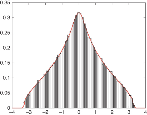
Figure 23.6
Comparison of the distribution of  according to our algorithm, with the histogram of eigenvalues for
  according to our algorithm, with the histogram of eigenvalues for
  , for
, for  .
.  are free semicircular elements and
  are independent standard Gaussian random matrices.
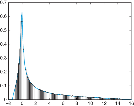
Figure 23.7
Comparison of the distribution of  according to our algorithm, with the histogram of eigenvalues for
  , for
, for  .
.  are of free Poisson elements, and
  are Wishart random matrices.
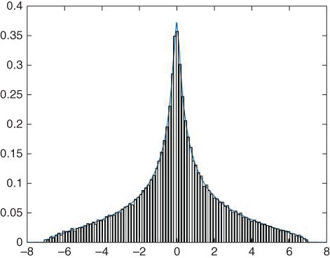
Figure 23.8
Comparison of the distribution of  according to our algorithm, with the histogram of eigenvalues for
  , for
, for  .
.  is of free semicircular elements and
  free Poisson ones.
  is an independent standard Gaussian random matrix, and
  is a Wishart matrix.

Figure 23.9
Comparison of the distribution of  according to our algorithm, with the histogram of eigenvalues for
  , for
, for  .
.  are of free Poisson elements, and
  are Wishart random matrices.

Figure 23.10
Comparison of the distribution of  according to our algorithm, with the histogram of eigenvalues for
  , for
, for  .
.  are of free Poisson elements, and
  are Wishart random matrices.
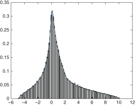
Figure 23.11
Comparison of the distribution of  according to our algorithm, with the histogram of eigenvalues for
  , for
, for  .
.  are of free semicircular elements and
  free Poisson ones.
  is an independent standard Gaussian random matrix, and
  is a Wishart matrix.
23.3 Applications to Smart Grids
In this section, we elaborate some of the more representative problems described in Section 23.1 that capture various features of interest in smart grids and we show how random matrix results have been used to tackle the problems that arise in the large power grid with wide deployment of PMU equipments. Besides, we also conclude with some state‐of‐art data driven methods for comparison.
23.3.1 Hypothesis Tests in Smart Grids
Considering the data model introduced in Section 23.2.1, the problem of testing hypotheses on means of populations and covariance matrices is addressed. We start with a review of traditional multivariate procedures for these tests. Then we develop adjustments of these procedures to handle high‐dimensional data in smart grids.
As depicted in Section 23.2.1, a large random matrix flow ![]() is adopted to represent the massive streaming PMU data in one sample period. Instead of analyzing the raw individual window‐truncated PMU data
is adopted to represent the massive streaming PMU data in one sample period. Instead of analyzing the raw individual window‐truncated PMU data ![]() [38, 39] or the statistic of
[38, 39] or the statistic of ![]() [52, 53], a comprehensive analysis of the statistic of
[52, 53], a comprehensive analysis of the statistic of ![]() is conducted in the following. More specifically, denote as
is conducted in the following. More specifically, denote as ![]() the covariance matrix of
the covariance matrix of ![]() th collected PMU measurements; we want to test the hypothesis:
th collected PMU measurements; we want to test the hypothesis:

It is worthy noting that the hypothesis (23.24) is a famous testing hypothesis in multivariate statistical analysis that aims to study samples share or approximately share some distribution and consider using a set of samples (data streams denoted in equation (23.4) in this paper), one from each population, to test the hypothesis that the covariance matrices of these populations are equal.
23.3.2 Data‐Driven Methods for State Evaluation
The LR test [69] and CLR test [70] as introduced in Section 23.3.1 are most commonly test statistics for the hypothesis in ( 23.24). These tests can be understood by replacing the population covariance matrix ![]() by its sample covariance matrix
by its sample covariance matrix ![]() . While direct substitution of
. While direct substitution of ![]() by
by ![]() brings invariance and good testing properties as shown in [ 69] for normally distributed data. The test statistic
brings invariance and good testing properties as shown in [ 69] for normally distributed data. The test statistic ![]() may not work for high‐dimensional data as demonstrated in [71, 72]. Besides, the estimator
may not work for high‐dimensional data as demonstrated in [71, 72]. Besides, the estimator ![]() has unnecessary terms, which slow down the convergence considerably when the dimension of PMU data is high [72, 73]. In such situations, to overcome the drawbacks, a trace criterion [ 72] is more suitable to the test problem. Specially, instead of estimating the population covariance matrix directly, a well‐defined distance measure exploiting the difference among data flow
has unnecessary terms, which slow down the convergence considerably when the dimension of PMU data is high [72, 73]. In such situations, to overcome the drawbacks, a trace criterion [ 72] is more suitable to the test problem. Specially, instead of estimating the population covariance matrix directly, a well‐defined distance measure exploiting the difference among data flow ![]() is conducted, that is, the trace‐based distance measure between
is conducted, that is, the trace‐based distance measure between ![]() and
and ![]() is
is
where ![]() is the trace operator. Instead of estimating
is the trace operator. Instead of estimating ![]() ,
, ![]() and
and ![]() by sample covariance matrix‐based estimators, we adopt the merits of the U‐statistics [74]. Especially, for
by sample covariance matrix‐based estimators, we adopt the merits of the U‐statistics [74]. Especially, for ![]() ,
,

is proposed to estimate ![]() . It is noted that
. It is noted that ![]() represents summation over mutually distinct indices. For example,
represents summation over mutually distinct indices. For example, ![]() says summation over the set
says summation over the set ![]() . Similarly, the estimator for
. Similarly, the estimator for ![]() can be expressed as
can be expressed as
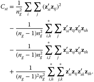
The test statistic that measures the distance between ![]() and
and ![]() is
is
Then the proposed test statistic can be expressed as:

As ![]() , the asymptotic normality [ 73] of the test statistic (23.28) is presented in the following:
, the asymptotic normality [ 73] of the test statistic (23.28) is presented in the following:
Let ![]() , the false alarm probability (FAP) for the proposed test statistic can be represented as
, the false alarm probability (FAP) for the proposed test statistic can be represented as
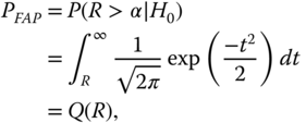
where ![]() . For a desired FAP
. For a desired FAP ![]() , the associated threshold should be chosen such that
, the associated threshold should be chosen such that
Otherwise, the detection rate (DR) can be denoted as
It is noted that the computation complexity of the proposed test statistic in (23.30) is ![]() which limits its practical application. Here, we proposed an effective approach to reduce the complexity of the proposed test statistic from
which limits its practical application. Here, we proposed an effective approach to reduce the complexity of the proposed test statistic from ![]() to
to ![]() by principal component calculation and redundant computation elimination. For simplicity, we briefly explained the technical details in our recent work, which is available at
by principal component calculation and redundant computation elimination. For simplicity, we briefly explained the technical details in our recent work, which is available at ![]() .
.
In this section, we evaluate the efficacy of the proposed test statistic for power system stability. For the experiments shown in the following, the real power flow data were of a chain‐reaction fault happened in the China power grids in 2013. The PMU number, the sample rate, and the total sample time are ![]() ,
, ![]() , and
, and ![]() , respectively. The chain‐reaction fault happened from
, respectively. The chain‐reaction fault happened from ![]() to
to ![]() . Let
. Let ![]() . Figure 23.12 shows that the mean and variance of
. Figure 23.12 shows that the mean and variance of ![]() agree well with theoretical ones. Based on the results in Figure 23.12 and event indicators (23.29), the occurrence time and the actual duration of the event can be identified as
agree well with theoretical ones. Based on the results in Figure 23.12 and event indicators (23.29), the occurrence time and the actual duration of the event can be identified as ![]() and
and ![]() , respectively. The location of the most sensitive bus can also be identified using the data analysis above. The result shown in Figure 23.13 illustrates that 17
, respectively. The location of the most sensitive bus can also be identified using the data analysis above. The result shown in Figure 23.13 illustrates that 17![]() and 18
and 18![]() PMU are the most sensitive PMUs, which is in accordance with the actual accident situation.
PMU are the most sensitive PMUs, which is in accordance with the actual accident situation.
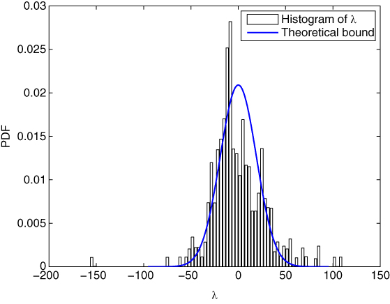
Figure 23.12 Parameter learning of the IEEE 118‐bus system.
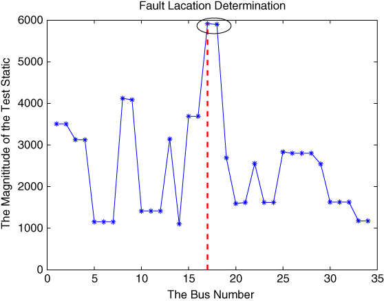
Figure 23.13 Data analysis of the realistic 34‐PMU power flow around events occurrence.
23.3.3 Situation Awareness based on Linear Eigenvalue Statistics
Situation awareness (SA) is of great significance in power system operation, and a reconsideration of SA is essential for future grids [ 24]. These future grids are always huge in size and complex in topology. Operating under a novel regulation, their management mode is much different from previous one.
All these driving forces demand a new prominence for the term “situation awareness” (SA). The SA is essential for power grid security; inadequate SA is identified as one of the root causes for the largest blackout in history—the August 14, 2003, blackout in the United States and Canada [75].
In [76], SA is defined as the perception of the elements in an environment, the comprehension of their meaning, and the projection of their status in the near future. This chapter is aimed at the use of model‐free and data‐driven methodology for the comprehension of the power grid.
The massive data compose the profile of the actual grid—present state; SA aims to translate the present state into perceived state for decision making [77].
The proposed methodology consists of three essential procedures as illustrated in Figure 23.14(b): (1) big data model—to model the system using experimental data for the RMM; (2) big data analysis—to conduct high‐dimensional analyses for the indicator system as the statistical solutions; (3) engineering interpretation—to visualize and interpret the statistical results for human beings for decision making.

Figure 23.14 SA and its methodology.
Power grids operate in a balance situation obeying

where ![]() and
and ![]() are the power injections on node
are the power injections on node ![]() , while
, while ![]() and
and ![]() are the injections of the network satisfying
are the injections of the network satisfying
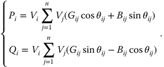
For simplicity, combining (23.33) and (23.34), we obtain
where ![]() is the vector of power injections on nodes depending on
is the vector of power injections on nodes depending on ![]() ,
, ![]() .
. ![]() is the system status variables depending on
is the system status variables depending on ![]() ,
, ![]() , while
, while ![]() is the network topology parameters depending on
is the network topology parameters depending on ![]() ,
, ![]() .
.
For a system state with certain fluctuations, and thus randomness in data sets, we formulate the system as
With a Taylor expansion, (23.36) is rewitten as

Equ. ( 23.34) shows that ![]() is linear with
is linear with ![]() ; it means that
; it means that ![]() . On the other hand, the values of system status variables
. On the other hand, the values of system status variables ![]() are relatively stable, and we can ignore the second‐order term
are relatively stable, and we can ignore the second‐order term ![]() and higher‐order terms. In this way, we turn (23.37) into
and higher‐order terms. In this way, we turn (23.37) into

Suppose the network topology is unchanged, i.e., ![]() . From (23.38), we deduce that
. From (23.38), we deduce that
On the other hand, suppose the power demand is unchanged, i.e., ![]() . From ( 23.38), we obtain that
. From ( 23.38), we obtain that
where ![]()
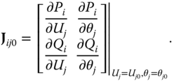
Note that ![]() , i.e., the inversion of the Jacobian matrix
, i.e., the inversion of the Jacobian matrix ![]() , expressed as
, expressed as
Thus, we describe the power system operation using a random matrix—if there is an unexpected active power change or short circuit, the corresponding change of system status variables ![]() , i.e.
, i.e. ![]() ,
, ![]() , will obey (23.39) or (23.40) respectively.
, will obey (23.39) or (23.40) respectively.
For a practical system, we can always build a relationship in the form of ![]() with a similar procedure as (23.35) to ( 23.40); it is linear in high dimensions. For an equilibrium operation system in which the reactive power is almost constant or changes much more slowly than the active one, the relationship model between voltage magnitude and active power is just like the multiple input multiple output (MIMO) model in wireless communication [49, 78]. Note that most variables of vector
with a similar procedure as (23.35) to ( 23.40); it is linear in high dimensions. For an equilibrium operation system in which the reactive power is almost constant or changes much more slowly than the active one, the relationship model between voltage magnitude and active power is just like the multiple input multiple output (MIMO) model in wireless communication [49, 78]. Note that most variables of vector ![]() are random due to the ubiquitous noises, e.g., small random fluctuations in
are random due to the ubiquitous noises, e.g., small random fluctuations in ![]() . In addition, we can add very small artificial fluctuations to make them random or replace the missing/bad data with random Gaussian variables. Furthermore, with the normalization, we can build the standard random matrix model (RMM) in the form of
. In addition, we can add very small artificial fluctuations to make them random or replace the missing/bad data with random Gaussian variables. Furthermore, with the normalization, we can build the standard random matrix model (RMM) in the form of ![]() , where
, where ![]() is a standard Gaussian random matrix.
is a standard Gaussian random matrix.
The data‐driven approach conducts analysis requiring no prior knowledge of system topologies, unit operation/control mechanism, causal relationship, etc. It is able to handle massive data all at once; the large size of the data, indeed, enhances the robustness of the final decision against the bad data (errors, losses, or asynchronization). Compared with classical data‐driven methodologies (e.g., PCA), the RMT‐based counterpart has some unique characteristics:
- The statistical indicator is generated from all the data in the form of matrix entries. This is not true for principal components—we really do not know the rank of the covariance matrix. Thus, the RMT approach is robust against those challenges in classical data‐driven methods, such as error accumulations and spurious correlations [ 53].
- For the statistical indicator, a theoretical or empirical value can be obtained in advance. The statistical indicator such as LES follows a Gaussian distribution, and its variance is bounded [79] and decays very fast in the order of
 given a moderate data dimension
  , say
, say 
- We can flexibly handle heterogenous data to realize data fusion via matrix operations, such as the blocking [80], the sum [ 78], the product [ 78], and the concatenation [ 53] of matrices. Data fusion is guided by the latest mathematical research [ 49, Chapter 7].
- Only eigenvalues are used for further analysis, while the eigenvectors are omitted. This leads to much smaller required memory space and faster data‐processing speed. Although some information is lost in this way, there is still rich information contained in the eigenvalues [81], especially those outliers [82, 83].
- Particularly, for a certain RMM, various forms of LES can be constructed by designing test functions without introducing any physical error (i.e.,
 ). Each LES, similar to a filter, provides a unique view angle. As a result, the system is systematically understood piece by piece. Finally, with a proper LES, we can trace some specific signal.
We adopt a standard IEEE 118‐node system as the grid network (Figure 23.15) and the events is shown in Table 23.1.

Figure 23.15 Partitioning network for the IEEE 118‐node system.
Table 23.1 Series of Events.
![]() is the power demand of node 52.
is the power demand of node 52.
| Stage | E1 | E2 | E3 | E4 |
| Time (s) |
|
|
|
|
|
|
0 |
|
|
|
The power demand of nodes are assigned as
where ![]() and
and ![]() are the element of a standard Gaussian random matrix;
are the element of a standard Gaussian random matrix; ![]() ,
, ![]() . Thus, the power demand on each node is obtained as the system injections (Figure 23.16(a)); the voltage can also be obtained (Figure 23.16(b)). Suppose we sample the voltage data at 1 Hz, and the data source is denoted as
. Thus, the power demand on each node is obtained as the system injections (Figure 23.16(a)); the voltage can also be obtained (Figure 23.16(b)). Suppose we sample the voltage data at 1 Hz, and the data source is denoted as ![]() . The number of dimensions is
. The number of dimensions is ![]() and the sampling time span is
and the sampling time span is ![]() .
.
Suppose that the power demand data (Fig. 23.16(a)) are unknown or unqualified for SA due to low sampling frequency or bad quality. For further analysis, we just start with data source ![]() (Figure 23.16(b)) and assign the analysis matrix as
(Figure 23.16(b)) and assign the analysis matrix as ![]() (4 minutes' time span). First, we conduct category for the system operation status; the results are shown as Figure 23.16(c). In general, according to the raw data source and the analysis matrix size, we divide our system into 8 stages. Note that it is a statistical division—
(4 minutes' time span). First, we conduct category for the system operation status; the results are shown as Figure 23.16(c). In general, according to the raw data source and the analysis matrix size, we divide our system into 8 stages. Note that it is a statistical division—![]() , and
, and ![]() are transition stages, and their time span is right equal to the length of the analysis matrix minus one, i.e,
are transition stages, and their time span is right equal to the length of the analysis matrix minus one, i.e, ![]() . These stages are described as follows:
. These stages are described as follows:
- For
 , the white noises play a dominant part. P
Node‐52 is rising in turn.
 - For
 , P
Node‐52 maintains stable growth.
 -
 , transition stage. Ramping signal exists.
 -
 , transition stages. Step signal exists.
 - For
 , voltage collapse.
We also select two typical data cross‐sections for stage ![]() and
and ![]() :
: ![]() during period
during period ![]() at the sampling time
at the sampling time ![]() , and 2)
, and 2) ![]() during period
during period ![]() at the sampling time
at the sampling time ![]() .
.
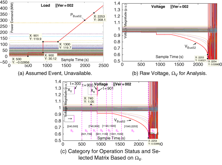
Figure 23.16 Assumed event, data source, and category for case.
Besides, as discussed in 23.2.1, we build up the RMM ![]() from the raw voltage data. Then,
from the raw voltage data. Then, ![]() is employed as a statistical indicator to conduct anomaly detection. For the selected data cross section
is employed as a statistical indicator to conduct anomaly detection. For the selected data cross section ![]() and
and ![]() , their M‐P law and ring law analysis are shown as Figure 23.17(a), 23.17(b), 23.17(c) and 23.17(d). With moving slide window (MSW), the
, their M‐P law and ring law analysis are shown as Figure 23.17(a), 23.17(b), 23.17(c) and 23.17(d). With moving slide window (MSW), the ![]() curve is obtained as Figure 23.17(e).
curve is obtained as Figure 23.17(e).
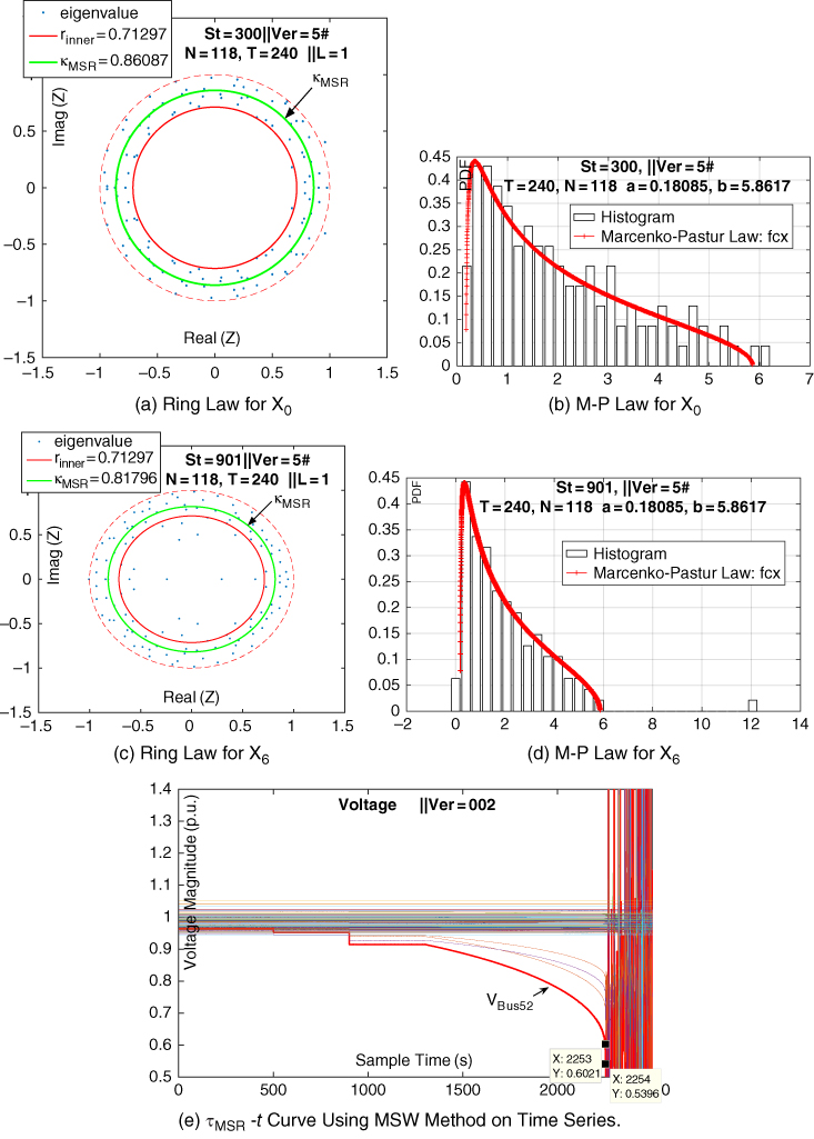
Figure 23.17 Anomaly detection result.

Figure 23.18 Illustration of various LES indicators.
Fig 23.17 shows that when there is no signal in the system, the experimental RMM well matches the ring law and M‐P law, and the experimental value of LES is approximately equal to the theoretical value. This validates the theoretical justification for modeling rapid fluctuation at each node with additive white Gaussian noise, as shown in Section 23.2.1. On the other hand, the ring law and M‐P law are violated at the very beginning (![]() ) of the step signal. Besides, the proposed high‐dimensional indicator
) of the step signal. Besides, the proposed high‐dimensional indicator ![]() , is extremely sensitive to the anomaly. At
, is extremely sensitive to the anomaly. At ![]() , the
, the ![]() starts the dramatic change as shown in the
starts the dramatic change as shown in the ![]() curve as Figure 23.17(e), while the raw voltage magnitudes are still in the normal range as shown in Figure 23.16(c). Moreover, we design numerous kinds of LES
curve as Figure 23.17(e), while the raw voltage magnitudes are still in the normal range as shown in Figure 23.16(c). Moreover, we design numerous kinds of LES ![]() and define
and define ![]() The results are shown in Figure 23.18 and prove that different indicators have different characteristics and effectiveness; this suggests another topic to explore in the future.
The results are shown in Figure 23.18 and prove that different indicators have different characteristics and effectiveness; this suggests another topic to explore in the future.
Furthermore, we investigate the SA based on the high‐dimensional spectrum test. The sampling time is set as ![]() and
and ![]() . The following Lemma 23.2.7 and Lemma 23.2.9,
. The following Lemma 23.2.7 and Lemma 23.2.9,
![]() (span
(span ![]() and
and ![]() ), and
), and ![]() (span
(span ![]() and
and ![]() ) are selected. The results are shown in Figure 23.19 and Fig. 23.20. These results validate that empirical spectral density test is competent to conduct anomaly detection—when the power grid is under a normal condition, the empirical spectral density
) are selected. The results are shown in Figure 23.19 and Fig. 23.20. These results validate that empirical spectral density test is competent to conduct anomaly detection—when the power grid is under a normal condition, the empirical spectral density ![]() and the ESD function
and the ESD function ![]() are almost strictly bounded between the upper bound and the lower bound of their asymptotic limits. On the other hand, these results also validate that GUE and LUE are proper mathematical tools to model the power grid operation.
are almost strictly bounded between the upper bound and the lower bound of their asymptotic limits. On the other hand, these results also validate that GUE and LUE are proper mathematical tools to model the power grid operation.
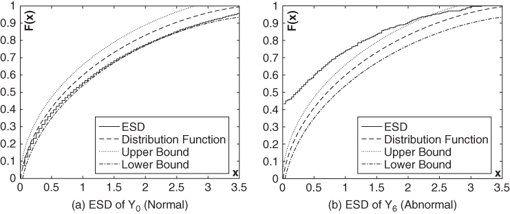
Figure 23.19 Anomaly detection using LUE matrices.
The ![]() curve (also called nose curve) and the smallest eigenvalue of the Jacobian matrix [ 39] are two clues for steady stability evaluation. In this case, we focus on the E4 part during which P
Node‐52 keep increasing to break down the steady stability. The related
curve (also called nose curve) and the smallest eigenvalue of the Jacobian matrix [ 39] are two clues for steady stability evaluation. In this case, we focus on the E4 part during which P
Node‐52 keep increasing to break down the steady stability. The related ![]() curve and
curve and ![]() curve, respectively, are given in Figure 23.21(a) and Figure 23.21(b). Only using the data source
curve, respectively, are given in Figure 23.21(a) and Figure 23.21(b). Only using the data source ![]() , we choose some data cross section,
, we choose some data cross section, ![]() as shown in Figure 23.21(a). The RMT‐based results are shown as Figure 23.22. The outliers become more evident as the stability degree decreases. The statistics of the outliers are similar to the smallest eigenvalue of the Jacobian matrix, Lyapunov exponent, or the entropy in some sense.
as shown in Figure 23.21(a). The RMT‐based results are shown as Figure 23.22. The outliers become more evident as the stability degree decreases. The statistics of the outliers are similar to the smallest eigenvalue of the Jacobian matrix, Lyapunov exponent, or the entropy in some sense.

Figure 23.20 Anomaly detection using GUE matrices.

Figure 23.21
The  curve and
  curve.
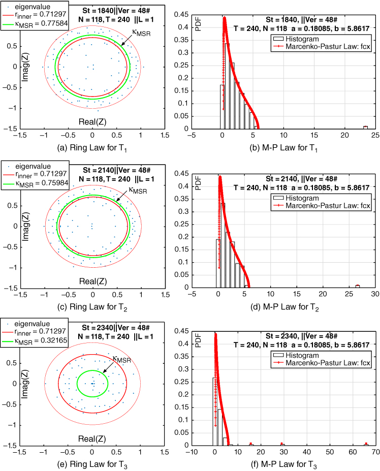
Figure 23.22 RMT‐based results for voltage stability evaluation.
For further analysis, we take the signal and stage division into account. Generally speaking, sorted by the stability degree, the stages are ordered as ![]() . According to Figure 23.18, we make Table 23.2. The high‐dimensional indicators
. According to Figure 23.18, we make Table 23.2. The high‐dimensional indicators ![]() and
and ![]() have the same trend as the stability degree order. These statistics have the potential for data‐driven stability evaluation.
have the same trend as the stability degree order. These statistics have the potential for data‐driven stability evaluation.
Table 23.2 Indicator of Various LESs at Each Stage.
| MSR | T2 | T3 | T4 | DET | LRF | |
|
|
||||||
|
|
0.8645 | 1338.3 | 10069 | 8.35E4 | 48.322 | 73.678 |
|
|
— | 665.26 | 93468 | 1.30E7 | 1.3532 | 1.4210 |
|
|
||||||
|
|
0.995 | 1.010 | 1.040 | 1.080 | 0.959 | 1.014 |
|
|
6E –6 | 78.38 | 3.03E4 | 7.14E6 | 0.4169 | 0.3908 |
|
|
1 | 1 | 1 | 1 | 1 | 1 |
|
|
||||||
|
|
0.9331 | 1.280 | 2.565 | 7.661 | 0.5453 | 1.284 |
|
|
1.49E1 | 1.64E2 | 1.16E3 | 8.63E3 | 3.43E1 | 3.97E1 |
|
|
||||||
|
|
0.9943 | 1.010 | 1.039 | 1.084 | 0.9568 | 1.015 |
|
|
0.8608 | 0.9121 | 0.9476 | 1.234 | 0.8972 | 1.101 |
|
|
||||||
|
|
0.8742 | 2.054 | 1.06E1 | 7.22E1 | 7E ‐2 | 1.597 |
|
|
5.49E1 | 2.06E3 | 3.87E4 | 8.54E5 | 1.52E2 | 1.62E2 |
|
|
||||||
|
|
0.9930 | 1.019 | 1.067 | 1.135 | 0.9488 | 1.021 |
|
|
0.7823 | 1.053 | 1.189 | 1.135 | 0.7310 | 0.9255 |
|
|
||||||
|
|
0.9337 | 1.295 | 2.787 | 9.615 | 0.5316 | 1.294 |
|
|
8.50E1 | 7.41E2 | 5.63E3 | 5.17E4 | 2.14E2 | 2.30E2 |
|
|
||||||
|
|
0.8906 | 1.717 | 6.530 | 3.48E1 | 0.1483 | 1.545 |
|
|
1.35E1 | 3.28E2 | 5.33E3 | 1.10E5 | 6.11E1 | 6.85E1 |
|
|
||||||
|
|
0.4259 | 1.02E1 | 2.11E2 | 4.65E3 | –1.4E1 | 1.08E1 |
|
|
1.94E3 | 5.81E5 | 1.20E8 | 3.2E10 | 9.02E4 | 9.62E4 |
a)
![]() ;
; ![]() .
.
The key for correlation analysis is the concatenated matrix ![]() , which consists of two parts—the basic matrix
, which consists of two parts—the basic matrix ![]() and a certain factor matrix
and a certain factor matrix ![]() , i.e.,
, i.e., ![]() . For more details, see our previous work [ 53]. The LES of each
. For more details, see our previous work [ 53]. The LES of each ![]() is computed in parallel, and Figure 23.23 shows the results.
is computed in parallel, and Figure 23.23 shows the results.

Figure 23.23 Sensitivity analysis based on concatenated matrix.
In Figure 23.23, the blue dotted line (marked with “None”) shows the LES of basic matrix ![]() , and the orange line (marked with “Random”) shows the LES of the concatenated matrix
, and the orange line (marked with “Random”) shows the LES of the concatenated matrix ![]() (
(![]() is the standard Gaussian random matrix). Figure 23.23 demonstrates that: (1) node 52 is the causing factor of the anomaly; (2) sensitive nodes are 51, 53, and 58; and (3) nodes 11, 45, 46, etc., are not affected by the anomaly. Based on this algorithm, we can continue to conduct behavior analysis, e.g., detection and estimation of residential PV installations [84]. Behavior analysis is a big topic. Because of space limitations, we will not expand it here.
is the standard Gaussian random matrix). Figure 23.23 demonstrates that: (1) node 52 is the causing factor of the anomaly; (2) sensitive nodes are 51, 53, and 58; and (3) nodes 11, 45, 46, etc., are not affected by the anomaly. Based on this algorithm, we can continue to conduct behavior analysis, e.g., detection and estimation of residential PV installations [84]. Behavior analysis is a big topic. Because of space limitations, we will not expand it here.
23.3.4 Early Event Detection Using Free Probability
![]() Following [85], we build the statistic model for power grids. Considering
Following [85], we build the statistic model for power grids. Considering ![]() random vectors observed at time instants
random vectors observed at time instants ![]() we form a random matrix as follows
we form a random matrix as follows
In an equilibrium operating system, the voltage magnitude vector injections ![]() with entries
with entries ![]() and the phase angle vector injections
and the phase angle vector injections ![]() with entries
with entries ![]() experience slight changes. Without dramatic topology changes, rich statistical empirical evidence indicates that the Jacobian matrix
experience slight changes. Without dramatic topology changes, rich statistical empirical evidence indicates that the Jacobian matrix ![]() keeps nearly constant, and so does
keeps nearly constant, and so does ![]() . Also, we can estimate the changes of
. Also, we can estimate the changes of ![]()
![]() and
and ![]() only with the classical approach. Thus, we rewrite (23.43) as:
only with the classical approach. Thus, we rewrite (23.43) as:
where ![]() ,
, ![]() and
and ![]() Here
Here ![]() and
and ![]() are random matrices. In particular,
are random matrices. In particular, ![]() is a random matrix with Gaussian entries.
is a random matrix with Gaussian entries.
![]() Multivariate linear or nonlinear polynomials perform a significant role in problem modeling, so we build our models on the basis of random matrix polynomials. Here, we study two typical random matrix polynomial models.
Multivariate linear or nonlinear polynomials perform a significant role in problem modeling, so we build our models on the basis of random matrix polynomials. Here, we study two typical random matrix polynomial models.
The first case is the multivariate linear polynomial:
The second one is the self‐adjoint multivariate nonlinear polynomial:
Here, both ![]() and
and ![]() are the sample covariance matrices. The asymptotic eigenvalue distributions of
are the sample covariance matrices. The asymptotic eigenvalue distributions of ![]() and
and ![]() can be obtained via basic principles of free probability theory, as introduced above. The asymptotic eigenvalue distributions of
can be obtained via basic principles of free probability theory, as introduced above. The asymptotic eigenvalue distributions of ![]() are regarded as the theoretical bounds.
are regarded as the theoretical bounds.
![]() We formulate our problem of anomaly detection in terms of the same hypothesis testing as [ 85]: no outlier exists
We formulate our problem of anomaly detection in terms of the same hypothesis testing as [ 85]: no outlier exists ![]() , and outlier exists
, and outlier exists ![]() .
.

where ![]() is the standard Gaussian random matrix.
is the standard Gaussian random matrix.
Generate ![]() ,
, ![]() from the sample data through the preprocess in 23.3.4. Compare the theoretical bound with the spectral distribution of raw data polynomials. If an outlier exists,
from the sample data through the preprocess in 23.3.4. Compare the theoretical bound with the spectral distribution of raw data polynomials. If an outlier exists, ![]() will be rejected, i.e., signals exist in the system.
will be rejected, i.e., signals exist in the system.
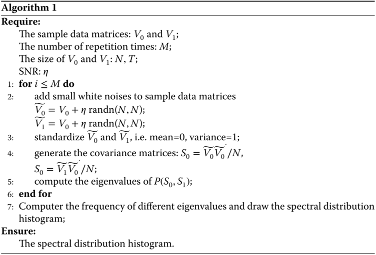
![]() The data sampled from the power grid is always non‐Gaussian, so we adopt a normalization procedure in [ 80] to conduct data preprocessing. Meanwhile, we employ the Monte Carlo method to compute the spectral distribution of the raw data polynomial according to asymptotic property theory. See details in Algorithm 1.
The data sampled from the power grid is always non‐Gaussian, so we adopt a normalization procedure in [ 80] to conduct data preprocessing. Meanwhile, we employ the Monte Carlo method to compute the spectral distribution of the raw data polynomial according to asymptotic property theory. See details in Algorithm 1.
![]() Our data fusion method is tested with simulated data in the standard IEEE 118‐bus system. Detailed information of the system refers to the case118.m in Matpower package and Matpower 4.1 User's Manual [86]. For all cases, let the sample dimension
Our data fusion method is tested with simulated data in the standard IEEE 118‐bus system. Detailed information of the system refers to the case118.m in Matpower package and Matpower 4.1 User's Manual [86]. For all cases, let the sample dimension ![]() . In our simulations, we set the sample length equal to
. In our simulations, we set the sample length equal to ![]() , i.e.,
, i.e., ![]() ,
, ![]() and select six sample voltage matrices presented in Table 23.3, as shown in Figure 23.24. The results of our simulations are presented in Figure 23.25 and Figure 23.26. The outliers existed when the system was abnormal, and its sizes become large when the anomaly becomes serious.
and select six sample voltage matrices presented in Table 23.3, as shown in Figure 23.24. The results of our simulations are presented in Figure 23.25 and Figure 23.26. The outliers existed when the system was abnormal, and its sizes become large when the anomaly becomes serious.
Table 23.3 System status and sampling data.
| Cross Section (s) | Sampling (s) | Descripiton |
|
|
|
Reference, no signal |
|
|
|
Existence of a step signal |
|
|
|
Steady load growth for Bus 22 |
|
|
|
Steady load growth for Bus 52 |
|
|
|
Chaos due to voltage collapse |
|
|
|
No signal |
a) We choose the temporal end edge of the sampling matrix as the marked time for the cross section. E.g., for ![]() , the temporal label is 217, which belongs to
, the temporal label is 217, which belongs to ![]() . Thus, this method is able to be applied to conduct real‐time analysis.
. Thus, this method is able to be applied to conduct real‐time analysis.

Figure 23.24 The event assumptions on time series.

Figure 23.25
Data fusion using multivariate linear polynomial  .
.

Figure 23.26
Data fusion using multivariate nonlinear polynomial  .
.
23.4 Conclusion and Future Directions
Motivated by the immediate demands of tackling the tricky problems raised from large‐scale smart grids, this chapter introduced RMT‐based schemes for spatiotemporal big data analysis. Firstly, we represent the spatiotemporal PMU data as a sequence of large random matrices. This is a crucial part for power state evaluation, as it turns the big PMU data into tiny data for practical uses. Rather than employing the raw PMU data, a comprehensive analysis of PMU data flow, namely, RMT‐based techniques, is then proposed to indicate the state evaluation. The core techniques include streaming PMU data modeling, asymptotic properties analysis, and data fusion methods (based on free probability). Besides, the case studies based on synthetic data and real data are also included with the aim to bridge the technology gap between RMT and spatiotemporal data analysis in smart grids.
The current work based on RMT provides a fundamental exploration of data analysis for spatiotemporal PMU data. Much more attention is to be paid to this research direction, such as classification of power events and load forecasting. It is also noted that this work provides data‐driven methods that are new substitutes for power system state estimation. The combination of power system scenario analysis, spectrum sensing mechanisms, networking protocols, and big data techniques [15, 34, 49, 87] is encouraged to be investigated for better understanding of the power system state.
References
- 1 US DOE. Grid 2030: A national vision for electricity's second 100 years. US DOE Report, 2003.
- 2 Santiago Grijalva and Muhammad Umer Tariq. Prosumer‐based smart grid architecture enables a flat, sustainable electricity industry. In Innovative Smart Grid Technologies (ISGT), 2011 IEEE PES, pages 1–6. IEEE, 2011.
- 3 Xiaoxin Zhou, Shuyong Chen, and Zongxiang Lu. Review and prospect for power system development and related technologies: a concept of three‐generation power systems. Proceedings of the CSEE, 33(22):1–11, Aug. 2013.
- 4 Shengwei Mei, Yuan Gong, and Feng LIU. The evolution model of three generation power systems and characteristic analysis. Proceedings of the CSEE, 7:1003–1012, 2014.
- 5 Xing He, Qian Ai, Zhiwen Yu, Yiting Xu, and Jian Zhang. Power system evolution and aggregation theory under the view of power ecosystem. Power System Protection and Control, 42(22):100–107, Nov. 2014.
- 6 Zhang Hong, Dongmei Zhao, Chenghong Gu, Furong Li, and Bo Wang. Economic optimization of smart distribution networks considering real‐time pricing. Journal of Modern Power Systems and Clean Energy, 2(4):350–356, 2014.
- 7 Yang Ji. Multi‐agent system based control of virtual power plant and its application in smart grid. Master's thesis, School of Electronic Information and Electrical Engineering, Shanghai Jiaotong University, 2011.
- 8 Xing He, Qian Ai, Peng Yuan, and Xiaohong Wang. The research on coordinated operation and cluster management for multi‐microgrids. In Sustainable Power Generation and Supply (SUPERGEN 2012), International Conference on, pages 1–3. IET, 2012.
- 9 Wilsun Xu and Jing Yong. Power disturbance data analytics–new application of power quality monitoring data. Proceedings of the CSEE, 33(19):93–101, July 2013.
- 10 IBM. The Four V's of Big Data. accessed date: July, 2015.
- 11 LS Moulin, AP Alves da Silva, MA El‐Sharkawi, et al. Support vector machines for transient stability analysis of large‐scale power systems. Power Systems, IEEE Transactions on, 19(2):818–825, 2004.
- 12 Yael Parag and Benjamin K Sovacool. Electricity market design for the prosumer era. Nature Energy, 1:16032, 2016.
- 13 C. Lynch. Big data: How do your data grow? Nature, 455(7209):28, 2008.
- 14 Science Staff. Dealing with data. challenges and opportunities. introduction. Science, 331(6018):692, 2011.
- 15 A. A Khan, M. H Rehmani, and M Reisslein. Cognitive radio for smart grids: Survey of architectures, spectrum sensing mechanisms, and networking protocols. IEEE Communications Surveys and Tutorials, 18(1):1–1, 2015.
- 16 Lei Chu, Robert Caiming Qiu, Xing He, Zenan Ling, and Yadong Liu. Massive streaming pmu data modeling and analytics in smart grid state evaluation based on multiple high‐dimensional covariance tests. IEEE Transactions on Big Data, PP(99):1–1, 2017.
- 17 Tómas A Brody, J Flores, J Bruce French, PA Mello, A Pandey, and Samuel SM Wong. Random‐matrix physics: spectrum and strength fluctuations. Reviews of Modern Physics, 53(3):385–480, 1981.
- 18 Laurent Laloux, Pierre Cizeau, Marc Potters, and Jean‐Philippe Bouchaud. Random matrix theory and financial correlations. International Journal of Theoretical and Applied Finance, 3(3):391–397, July 2000.
- 19 Hsinchun Chen, Roger HL Chiang, and Veda C Storey. Business intelligence and analytics: From big data to big impact. MIS quarterly, 36(4):1165–1188, 2012.
- 20 Doug Howe, Maria Costanzo, Petra Fey, Takashi Gojobori, Linda Hannick, Winston Hide, David P Hill, Renate Kania, Mary Schaeffer, Susan St Pierre, et al. Big data: The future of biocuration. Nature, 455(7209):47–50, 2008.
- 21 Robert Qiu and Michael Wicks. Cognitive Networked Sensing and Big Data. Springer, 2013.
- 22 C. Zhang and R. C. Qiu. Data modeling with large random matrices in a cognitive radio network testbed: Initial experimental demonstrations with 70 nodes. ArXiv e‐prints, Apr. 2014.
- 23 Xia Li, Feng Lin, and Robert C Qiu. Modeling massive amount of experimental data with large random matrices in a real‐time UWB‐MIMO system. ArXiv e‐prints, Apr. 2014.
- 24 T. Hong, C. Chen, J. Huang, et al. Guest editorial big data analytics for grid modernization. IEEE Transactions on Smart Grid, 7(5):2395–2396, Sept 2016.
- 25 M. Rafferty, X. Liu, D. M. Laverty, and S. McLoone. Real‐time multiple event detection and classification using moving window pca. IEEE Transactions on Smart Grid, 7(5):2537–2548, Sept 2016.
- 26 H. Jiang, X. Dai, D. W. Gao, J. J. Zhang, Y. Zhang, and E. Muljadi. Spatial‐temporal synchrophasor data characterization and analytics in smart grid fault detection, identification, and impact causal analysis. IEEE Transactions on Smart Grid, 7(5):2525–2536, Sept 2016.
- 27 H. Sun, Z. Wang, J. Wang, Z. Huang, N. Carrington, and J. Liao. Data‐driven power outage detection by social sensors. IEEE Transactions on Smart Grid, 7(5):2516–2524, Sept 2016.
- 28 X. Zhang and S. Grijalva. A data‐driven approach for detection and estimation of residential pv installations. IEEE Transactions on Smart Grid, 7(5):2477–2485, Sept 2016.
- 29 H. Shaker, H. Zareipour, and D. Wood. A data‐driven approach for estimating the power generation of invisible solar sites. IEEE Transactions on Smart Grid, 7(5):2466–2476, Sept 2016.
- 30 B. Wang, B. Fang, Y. Wang, H. Liu, and Y. Liu. Power system transient stability assessment based on big data and the core vector machine. IEEE Transactions on Smart Grid, 7(5):2561–2570, Sept 2016.
- 31 AG Phadke and Rui Menezes de Moraes. The wide world of wide‐area measurement. Power and Energy Magazine, IEEE, 6(5):52–65, 2008.
- 32 Vladimir Terzija, Gustavo Valverde, Deyu Cai, Pawel Regulski, Vahid Madani, John Fitch, Srdjan Skok, Miroslav M Begovic, and Arun Phadke. Wide‐area monitoring, protection, and control of future electric power networks. Proceedings of the IEEE, 99(1):80–93, 2011.
- 33 Le Xie, Yang Chen, and Huaiwei Liao. Distributed online monitoring of quasi‐static voltage collapse in multi‐area power systems. Power Systems, IEEE Transactions on, 27(4):2271–2279, 2012.
- 34 Athar Ali Khan, Mubashir Husain Rehmani, and Martin Reisslein. Requirements, design challenges, and review of routing and mac protocols for cr‐based smart grid systems. IEEE Communications Magazine, 55(5):206–215, 2017.
- 35 Quanyuan Jiang, Xingpeng Li, Bo Wang, and Haijiao Wang. Pmu‐based fault location using voltage measurements in large transmission networks. Power Delivery, IEEE Transactions on, 27(3):1644–1652, 2012.
- 36 Mahesh Venugopal and Chetan Tiwari. A novel algorithm to determine fault location in a transmission line using pmu measurements. In Smart Instrumentation, Measurement and Applications (ICSIMA), 2013 IEEE International Conference on, pages 1–4. IEEE, 2013.
- 37 Ali H Al‐Mohammed and MA Abido. A fully adaptive pmu‐based fault location algorithm for series‐compensated lines. Power Systems, IEEE Transactions on, 29(5):2129–2137, 2014.
- 38 Le Xie, Yang Chen, and PR Kumar. Dimensionality reduction of synchrophasor data for early event detection: Linearized analysis. IEEE Transactions on Power Systems, 29(6):2784–2794, 2014.
- 39 Jong Min Lim and Christopher L DeMarco. Svd‐based voltage stability assessment from phasor measurement unit data. IEEE Transactions on Power Systems, 31(4):2557–2565, 2016.
- 40 Eugene P Wigner. Lower limit for the energy derivative of the scattering phase shift. Physical Review, 98(1):145, 1955.
- 41 Eugene P. Wigner. On the distribution of the roots of certain symmetric matrices. Annals of Mathematics, 67(2):325–327, 1958.
- 42 Eugene P Wigner. The problem of measurement. American Journal of Physics, 31(1):6–15, 1963.
- 43 Eugene P. Wigner. Random matrices in physics. Siam Review, 9(1):1–23, 1967.
- 44 Eugene P. Wigner. Characteristic Vectors of Bordered Matrices with Infinite Dimensions I. Springer Berlin Heidelberg, 1993.
- 45 V. A. Marchenko and L. A. Pastur. Distribution of eigenvalues for some sets of random matrices. Mathematics of the USSR‐Sbornik, 1(1):507–536, 1967.
- 46 Guionnet, Krishnapur, Manjunath, Zeitouni, and Ofer. The single ring theorem. Annals of Mathematics, 174(2):1189–1217, 2009.
- 47 Greg W. Anderson, Alice Guionnet, and Ofer Zeitouni. An introduction to random matrices. Cambridge Studies in Advanced Mathematics, 2009.
- 48 Terence Tao. Topics in Random Matrix Theory. American Mathematical Society, 2012.
- 49 R Qiu and P Antonik. Smart Grid and Big Data. John Wiley and Sons, 2015.
- 50 Math HJ Bollen. Understanding power quality problems, volume 3. IEEE press New York, 2000.
- 51 Denis Hau Aik Lee. Voltage stability assessment using equivalent nodal analysis. IEEE Transactions on Power Systems, 31(1):454–463, 2016.
- 52 Goodarz Ghanavati, Paul DH Hines, and Taras I Lakoba. Identifying useful statistical indicators of proximity to instability in stochastic power systems. IEEE Transactions on Power Systems, 31(2):1360–1368, 2016.
- 53 Xinyi Xu, Xing He, Qian Ai, and Robert Caiming Qiu. A correlation analysis method for power systems based on random matrix theory. IEEE Transactions on Smart Grid, PP(99):1–10, 2015.
- 54 Rudolf Wegmann. The asymptotic eigenvalue‐distribution for a certain class of random matrices. Journal of Mathematical Analysis and Applications, 56(1):113–132, 1976.
- 55 Robert Caiming Qiu, Zhen Hu, Husheng Li, and Michael C Wicks. Cognitive radio communication and networking: Principles and practice. John Wiley & Sons, 2012.
- 56 Yingshuang Cao, Long Cai, C Qiu, Jie Gu, Xing He, Qian Ai, and Zhijian Jin. A random matrix theoretical approach to early event detection using experimental data. arXiv preprint arXiv:1503.08445, 2015.
- 57 M. L. Mehta. Random matrices, volume 142. Academic press, 2004.
- 58 Z. Bai. Convergence rate of expected spectral distributions of large random matrices. part i. wigner matrices. The Annals of Probability, pages 625–648, 1993.
- 59 Z. Bai, B. Miao, and J. Tsay. A note on the convergence rate of the spectral distributions of large random matrices. Statistics & Probability Letters, 34(1):95–101, 1997.
- 60 F. Götze and A. Tikhomirov. Rate of convergence to the semi‐circular law. Probability Theory and Related Fields, 127(2):228–276, 2003.
- 61 Z. Bai, B. Miao, and J. Yao. Convergence rates of spectral distributions of large sample covariance matrices. SIAM journal on matrix analysis and applications, 25(1):105–127, 2003.
- 62 V. L. Girko. Extended proof of the statement: Convergence rate of the expected spectral functions of symmetric random matrices is equal to o () and the method of critical steepest descent. Random Operators and Stochastic Equations, 10(3):253–300, 2002.
- 63 Friedrich Götze and Alexander Tikhomirov. The rate of convergence for spectra of gue and lue matrix ensembles. Open Mathematics, 3(4):666–704, 2005.
- 64 Voiculescu Dan. Symmetries of some reduced free product C*‐algebras. Springer Berlin Heidelberg, 1985.
- 65 Voiculescu Dan. Limit laws for random matrices and free products. Inventiones mathematicae, 104(1):201–220, 1991.
- 66 Serban Belinschi, Tobias Mai, and Roland Speicher. Analytic subordination theory of operator‐valued free additive convolution and the solution of a general random matrix problem. Journal Für Die Reine Und Angewandte Mathematik, 2013.
- 67 Roland Speicher and Roland Speicher. Polynomials in asymptotically free random matrices. Acta Physica Polonica, 46(9), 2015.
- 68 Greg W. Anderson. Convergence of the largest singular value of a polynomial in independent wigner matrices. Annals of Probability, 38(1):110–C112, 2011.
- 69 Zhidong Bai and Hewa Saranadasa. Effect of high dimension: by an example of a two sample problem. Statistica Sinica, pages 311–329, 1996.
- 70 Zhidong Bai, Dandan Jiang, Jian‐Feng Yao, and Shurong Zheng. Corrections to lrt on large‐dimensional covariance matrix by rmt. The Annals of Statistics, pages 3822–3840, 2009.
- 71 Olivier Ledoit and Michael Wolf. Some hypothesis tests for the covariance matrix when the dimension is large compared to the sample size. Annals of Statistics, pages 1081–1102, 2002.
- 72 Song Xi Chen and Ying‐Li Qin. A two‐sample test for high‐dimensional data with applications to gene‐set testing. The Annals of Statistics, 38(2):808–835, 2010.
- 73 Song Xi Chen, Li‐Xin Zhang, and Ping‐Shou Zhong. Tests for high‐dimensional covariance matrices. Journal of the American Statistical Association, 2012.
- 74 AJ Lee. U‐statistics. Theory and Practice,'' Marcel Dekker, New York, 1990.
- 75 US‐Canada Power System Outage Task Force, Spencer Abraham, Herb Dhaliwal, R John Efford, Linda J Keen, Anne McLellan, John Manley, Kenneth Vollman, Nils J Diaz, Tom Ridge, et al. Final report on the August 14, 2003 blackout in the United states and Canada: causes and recommendations. US‐Canada Power System Outage Task Force, 2004.
- 76 Mica R Endsley. Designing for situation awareness: An approach to user‐centered design. CRC Press, 2011.
- 77 Mathaios Panteli, Peter Crossley, Daniel S Kirschen, Dejan J Sobajic, et al. Assessing the impact of insufficient situation awareness on power system operation. Power Systems, IEEE Transactions on, 28(3):2967–2977, 2013.
- 78 Changchun Zhang and Robert C Qiu. Massive mimo as a big data system: Random matrix models and testbed. IEEE Access, 3:837–851, 2015.
- 79 Mariya Shcherbina. Central limit theorem for linear eigenvalue statistics of the wigner and sample covariance random matrices. ArXiv e‐prints, January 2011.
- 80 Xing He, Qian Ai, Robert Caiming Qiu, and Wentao Huang. A big data architecture design for smart grids based on random matrix theory. IEEE Transactions on Smart Grid, 32(3):1, 2015.
- 81 Jesper R Ipsen and Mario Kieburg. Weak commutation relations and eigenvalue statistics for products of rectangular random matrices. Physical Review E, 89(3), 2014. Art. ID 032106.
- 82 Florent Benaych‐Georges and Jean Rochet. Outliers in the single ring theorem. Probability Theory and Related Fields, pages 1–51, May 2015.
- 83 Terence Tao. Outliers in the spectrum of iid matrices with bounded rank perturbations. Probability Theory and Related Fields, 155(1‐2):231–263, 2013.
- 84 Xiaochen Zhang and Santiago Grijalva. A data‐driven approach for detection and estimation of residential pv installations. IEEE Transactions on Smart Grid, 7(5):2477–2485, 2016.
- 85 Xing He, Robert Caiming Qiu, Qian Ai, Lei Chu, Xinyi Xu, and Zenan Ling. Designing for situation awareness of future power grids: An indicator system based on linear eigenvalue statistics of large random matrices. IEEE Access, 4:3557–3568, 2016.
- 86 Ray D Zimmerman and Carlos E Murillo‐Sánchez. Matpower 4.1 user's manual. Power Systems Engineering Research Center, 2011.
- 87 Robert Qiu and Michael Wicks. Cognitive networked sensing and big data. Springer, 2014.
