Chapter 7
Differentiation Problems
IN THIS CHAPTER
![]() Position, velocity, and acceleration — VROOOOM
Position, velocity, and acceleration — VROOOOM
![]() Related rates — brace yourself
Related rates — brace yourself
![]() Standing in line for linear approximations
Standing in line for linear approximations
In this chapter I finally get around to showing you how to use calculus to solve some practical problems.
Optimization Problems
One practical use of differentiation is finding the maximum or minimum value of a real-world function: the maximum output of a factory or range of a missile, the minimum time to accomplish some task, and so on. Here’s an example.
The maximum area of a corral
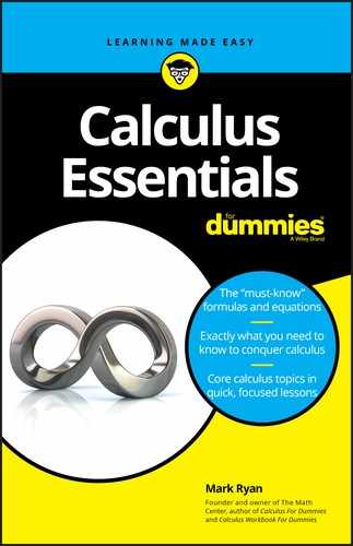
A rancher can afford 300 feet of fencing to build a corral that’s divided into two equal rectangles. See Figure 7-1. What dimensions will maximize the corral’s area?
1.a. Express the thing you want maximized, the area, as a function of the two unknowns, x and y.
In some optimization problems, you can write the thing you’re trying to maximize or minimize as a function of one variable — which is always what you want. But here, the area is a function of two variables, so Step 1 has two additional substeps.
1.b. Use the given information to relate the two unknowns to each other.
The fencing is used for seven sections, thus
1.c. Solve this equation for y and plug the result into the y in the equation from Step 1.a. This gives you what you need — a function of one variable.
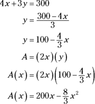
2. Determine the domain of the function.
You can’t have a negative length of fence, so x can’t be negative, and the most x can be is 300 divided by 4, or 75. Thus, ![]() . You now want to find the maximum value of
. You now want to find the maximum value of ![]() in this interval. You use the method from Chapter 6’s “Finding Absolute Extrema on a Closed Interval.”
in this interval. You use the method from Chapter 6’s “Finding Absolute Extrema on a Closed Interval.”
3. Find the critical numbers of ![]() in the open interval (0, 75) by setting its derivative equal to zero and solving. And don’t forget to check for numbers where the derivative is undefined.
in the open interval (0, 75) by setting its derivative equal to zero and solving. And don’t forget to check for numbers where the derivative is undefined.
Because ![]() is defined for all x-values, 37.5 is the only critical number.
is defined for all x-values, 37.5 is the only critical number.
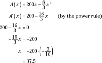
4. Evaluate the function at the critical number, 37.5, and at the endpoints of the interval, 0 and 75.

FIGURE 7-1: Calculus for cowboys — maximizing a corral.
 The min or max you want isn’t often at an endpoint, but it can be, so be sure to evaluate the function at the interval’s two endpoints.
The maximum value in the interval is 3,750, and thus, an x-value of 37.5 feet maximizes the corral’s area. The length is 2x, or 75 feet. The width is y, which equals ![]() . Plugging in 37.5 gives you
. Plugging in 37.5 gives you ![]() , or 50 feet. So the rancher will build a 75'×50' corral with an area of 3,750 square feet.
, or 50 feet. So the rancher will build a 75'×50' corral with an area of 3,750 square feet.
Position, Velocity, and Acceleration
Every time you get in your car, you witness differentiation first hand. Your speed is the first derivative of your position. And when you accelerate or decelerate, you experience a second derivative.
 If a function gives the position of something as a function of time, the first derivative gives its velocity, and the second derivative gives its acceleration. So, you differentiate position to get velocity, and you differentiate velocity to get acceleration.
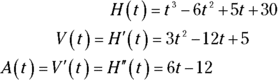
Here’s an example: A yo-yo moves straight up and down. Its height above the ground, as a function of time, is given by the function ![]() , where t is in seconds and
, where t is in seconds and ![]() is in inches.
is in inches. ![]() , it’s 30 inches above the ground, and after 4 seconds, it’s at a height of 18 inches. Velocity,
, it’s 30 inches above the ground, and after 4 seconds, it’s at a height of 18 inches. Velocity, ![]() , is the derivative of position (height in this problem), and acceleration,
, is the derivative of position (height in this problem), and acceleration, ![]() , is the derivative of velocity. Thus —
, is the derivative of velocity. Thus —
Take a look at the graphs of these three functions in Figure 7-2.

FIGURE 7-2: The graphs of the yo-yo’s height, velocity, and acceleration functions from 0 to 4 seconds.
Using the three functions and their graphs, I want to discuss several things about the yo-yo’s motion:
- Maximum and minimum height
- Maximum, minimum, and average velocity
- Total displacement
- Maximum, minimum, and average speed
- Total distance traveled
- Positive and negative acceleration
- Speeding up and slowing down
That’s a lot to cover, so I’m going to cut some corners — like not always checking endpoints when looking for extrema if it’s obvious they don’t occur there. But before discussing the bullet points, let’s go over a few things about velocity, speed, and acceleration.
Velocity versus speed
Your friends won’t complain — or even notice — if you use the words “velocity” and “speed” interchangeably, but your friendly mathematician will complain. Here’s the difference.
For the velocity function in Figure 7-2, upward motion is defined as a positive velocity, and downward motion is a negative velocity — this is the standard way velocity is treated in most calculus and physics problems. (If the motion is horizontal, going right is a positive velocity and going left is a negative velocity.)
Speed, on the other hand, is always positive (or zero). If a car goes by at 50 mph, for instance, you say its speed is 50, and you mean positive 50, regardless of whether it’s going to the right or the left. For velocity, the direction matters; for speed it doesn’t. In everyday life, speed is a simpler idea than velocity because it agrees with common sense. But in calculus, speed is actually the trickier idea because it doesn’t fit nicely into the three-function scheme shown in Figure 7-2.
You’ve got to keep the velocity-speed distinction in mind when analyzing velocity and acceleration. For example, if an object is going down (or to the left) faster and faster, its speed is increasing, but its velocity is decreasing because its velocity is becoming a bigger negative (and bigger negatives are smaller numbers). This seems weird, but that’s the way it works. And here’s another strange thing: Acceleration is defined as the rate of change of velocity, not speed. So, if an object is slowing down while going in the downward direction, and thus has an increasing velocity — because the velocity is becoming a smaller negative — the object has a positive acceleration. In everyday English, you’d say the object is decelerating (slowing down), but in calculus class, you say that the object has a negative velocity and a positive acceleration. (By the way, “deceleration” isn’t exactly a technical term, so you should probably avoid it in calculus class. It’s best to use the following vocabulary: “positive acceleration,” “negative acceleration,” “speeding up,” and “slowing down.” More on these things later.)
Maximum and minimum height
The maximum and minimum of ![]() occur at the local extrema seen in Figure 7-2. To locate them, set the derivative of
occur at the local extrema seen in Figure 7-2. To locate them, set the derivative of ![]() , that’s
, that’s ![]() , equal to zero and solve.
, equal to zero and solve.
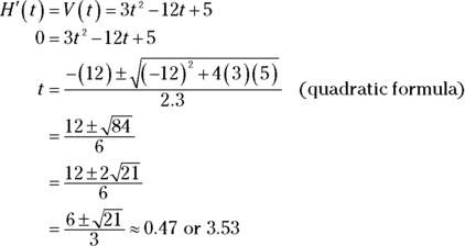
These two numbers are the zeros of ![]() and the t-coordinates (time-coordinates) of the max and min of
and the t-coordinates (time-coordinates) of the max and min of ![]() , which you can see in Figure 7-2. In other words, these are the times when the yo-yo reaches its maximum and minimum heights. Plug these numbers into
, which you can see in Figure 7-2. In other words, these are the times when the yo-yo reaches its maximum and minimum heights. Plug these numbers into ![]() to obtain the heights:
to obtain the heights:
So the yo-yo gets as high as about 31.1 inches above the ground at ![]() second and as low as about 16.9 inches at
second and as low as about 16.9 inches at ![]() seconds.
seconds.
Velocity and displacement
Again, speed is always positive, but going down (or left) is a negative velocity. The connection between displacement and distance traveled is similar: Distance traveled is always positive (or zero), but going down (or left) is a negative displacement. The basic idea is this: If you drive to a store 1 mile away — taking the scenic route and clocking 3 miles on your odometer — your total distance traveled is 3 miles, but your displacement is just 1 mile.
Total displacement
Total displacement equals final position minus initial position. So, because the yo-yo starts at a height of 30 and ends at a height of 18,
This is negative because the net movement is downward.
Average velocity
Average velocity is given by total displacement divided by elapsed time. Thus,
This negative answer tells you that the yo-yo, on average, is going down 3 inches per second.
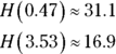
Maximum and minimum velocity
To determine the yo-yo’s maximum and minimum velocity during the interval from 0 to 4 seconds, set the derivative of ![]() , that’s
, that’s ![]() , equal to zero and solve:
, equal to zero and solve:
Now, evaluate ![]() at the critical number, 2, and at the interval’s endpoints, 0 and 4:
at the critical number, 2, and at the interval’s endpoints, 0 and 4:

The yo-yo has a maximum velocity of 5 inches per second twice — at the beginning and the end of the interval. It reaches a minimum velocity of ![]() inches per second at
inches per second at ![]() seconds.
seconds.
Speed and distance traveled
Unlike velocity and displacement, which have technical definitions, speed and distance traveled have commonsense meanings. Speed, of course, is what you read on your speedometer, and you can read distance traveled on your odometer or “tripometer.”
Total distance traveled
To determine total distance, add the distances traveled on each leg of the yo-yo’s trip: the up leg, the down leg, and the second up leg.
First, the yo-yo goes up from a height of 30 inches to about 31.1 inches (where the first turn-around point is), a distance of about 1.1 inches. Next, it goes down from about 31.1 to about 16.9 (the height of the second turn-around point). That’s 31.1 – 16.9, or about 14.2 inches. Finally, it goes up again from about 16.9 to its final height of 18 inches, another 1.1 inches. Add the three distances to get total distance travelled: ![]() inches.
inches.
Average speed
The yo-yo’s average speed is given by the total distance traveled divided by the elapsed time. Thus,
Maximum and minimum speed
You previously determined the yo-yo’s maximum velocity (5 inches per second) and its minimum velocity (![]() inches per second). A velocity of
inches per second). A velocity of ![]() is a speed of 7, so that’s the yo-yo’s maximum speed. Its minimum speed of zero occurs at the two turnaround points.
is a speed of 7, so that’s the yo-yo’s maximum speed. Its minimum speed of zero occurs at the two turnaround points.
 For a continuous velocity function, the minimum speed is zero whenever the maximum and minimum velocities are of opposite signs or when one of them is zero. When the maximum and minimum velocities are both positive or both negative, then the minimum speed is the lesser of the absolute values of the maximum and minimum velocities. In all cases, the maximum speed is the greater of the absolute values of the maximum and minimum velocities. Is that a mouthful or what?
Acceleration
Let’s go over acceleration: Put your pedal to the metal.
Positive and negative acceleration
The graph of the acceleration function at the bottom of Figure 7-2 is a simple line, ![]() . It’s easy to see that the acceleration of the yo-yo goes from a minimum of
. It’s easy to see that the acceleration of the yo-yo goes from a minimum of ![]() at
at ![]() seconds to a maximum of 12
seconds to a maximum of 12 ![]() at
at ![]() seconds, and that the acceleration is zero at
seconds, and that the acceleration is zero at ![]() when the yo-yo reaches its minimum velocity (and maximum speed). When the acceleration is negative — on the interval [0, 2) — that means that the velocity is decreasing. When the acceleration is positive — on the interval (2, 4] — the velocity is increasing.
when the yo-yo reaches its minimum velocity (and maximum speed). When the acceleration is negative — on the interval [0, 2) — that means that the velocity is decreasing. When the acceleration is positive — on the interval (2, 4] — the velocity is increasing.
Speeding up and slowing down
Figuring out when the yo-yo is speeding up and slowing down is probably more interesting and descriptive of its motion than the info in the preceding section. An object is speeding up (what we call “acceleration” in everyday speech) whenever the velocity and the calculus acceleration are both positive or both negative. And an object is slowing down (what we call “deceleration”) when the velocity and the calculus acceleration are of opposite signs.
Look at all three graphs in Figure 7-2 again. From ![]() to about
to about ![]() (when velocity is zero), the velocity is positive and the acceleration is negative, so the yo-yo is slowing down (till it reaches its maximum height). When
(when velocity is zero), the velocity is positive and the acceleration is negative, so the yo-yo is slowing down (till it reaches its maximum height). When ![]() , the deceleration is greatest (12
, the deceleration is greatest (12 ![]() ; the graph shows negative 12, but I’m calling it positive 12 because I’m calling it a deceleration, get it?) From about
; the graph shows negative 12, but I’m calling it positive 12 because I’m calling it a deceleration, get it?) From about ![]() to
to ![]() , both velocity and acceleration are negative, so the yo-yo is speeding up. From
, both velocity and acceleration are negative, so the yo-yo is speeding up. From ![]() to about
to about ![]() , velocity is positive and acceleration is negative, so the yo-yo is slowing down again (till it bottoms out at its lowest height). Finally, from about
, velocity is positive and acceleration is negative, so the yo-yo is slowing down again (till it bottoms out at its lowest height). Finally, from about ![]() to
to ![]() , both velocity and acceleration are positive, so the yo-yo is speeding up again. The yo-yo reaches its greatest acceleration of 12
, both velocity and acceleration are positive, so the yo-yo is speeding up again. The yo-yo reaches its greatest acceleration of 12 ![]() at
at ![]() seconds.
seconds.
Tying it all together
Note the following connections among the three graphs in Figure 7-2. The negative section on the graph of ![]() — from
— from ![]() to
to ![]() — corresponds to a decreasing section of the graph of
— corresponds to a decreasing section of the graph of ![]() and a concave down section of the graph of
and a concave down section of the graph of ![]() . The positive interval on the graph of
. The positive interval on the graph of ![]() — from
— from ![]() to
to ![]() — corresponds to an increasing interval on the graph of
— corresponds to an increasing interval on the graph of ![]() and a concave up interval on the graph of
and a concave up interval on the graph of ![]() . When
. When ![]() seconds,
seconds, ![]() has a zero,
has a zero, ![]() has a local minimum, and
has a local minimum, and ![]() has an inflection point.
has an inflection point.
Related Rates
Say you’re filling up your swimming pool; you know how fast water is coming out of your hose, and you want to calculate how fast the water level in the pool is rising. You know one rate (how fast the water is pouring in), and you want to determine another rate (how fast the water level is rising). These rates are called related rates because one depends on the other — the faster the water is poured in, the faster the water level rises. In a typical related rates problem, the rate or rates you’re given are unchanging, but the rate you have to figure out is changing with time. You have to determine this rate at one particular point in time.
A calculus crossroads
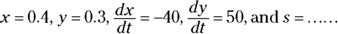
One car leaves an intersection traveling north at 50 mph; another is driving west toward the intersection at 40 mph. At one point, the north-bound car is three-tenths of a mile north of the intersection and the west-bound car is four-tenths of a mile east of it. At this point, how fast is the distance between the cars changing?
-
Draw a diagram and label it with any unchanging measurements (there are none in this particular problem), and make sure to assign a variable to anything in the problem that’s changing (unless it’s irrelevant to the problem). See Figure 7-3.
Note that variables have been assigned to the distance between Car A and the intersection, the distance between Car B and the intersection, and the distance between the two cars, because those are changing distances. The 0.3 and 0.4 are in parentheses to emphasize that they’re not unchanging measurements; they’re the distances at one particular point in time.
 In related rates problems, it’s important to distinguish between what is changing and what is not changing. You may run across a similar problem in your calculus textbook. It involves a ladder leaning against and sliding down a wall. The diagram for this problem would be very similar to Figure 7-3 except that the y-axis would represent the wall, the x-axis would be the ground, and the diagonal line would be the ladder. Despite the similarities between these two problems, there’s an important difference: The distance between the cars is changing, so the diagonal line in Figure 7-3 is labeled with a variable, s. A ladder, on the other hand, has a fixed length, so the diagonal line in the diagram for the ladder problem would be labeled with a number, not a variable.
 -
List all given rates and the rate you’re asked to determine as derivatives with respect to time.
As Car A travels north, y is growing at 50 miles per hour. That’s a rate, a change in distance per change in time. So,
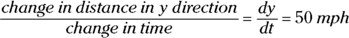
As Car B travels west, x is shrinking at 40 miles per hour. That’s a negative rate:
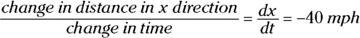
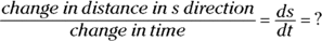
You have to figure out how fast s is changing, so
-
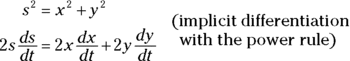
Write the formula that relates the variables in the problem: x, y, and s.
There’s a right triangle in your diagram, so you use the Pythagorean Theorem:
 . The Pythagorean Theorem is used a lot in related rates problems. If there’s a right triangle in your problem, it’s likely that
  is the formula you’ll need.
 -
Differentiate your formula with respect to time, t.
When you differentiate in a related rates problem, all variables are treated like the ys are treated in a typical implicit differentiation problem.
- Substitute known values for the rates and variables in the equation from Step 4, and then solve for the thing you’re asked to determine,
 .
. 
There’s a glitch here because you don’t know s (you’ll run into this glitch in some but not all related rates problems). No worries, just use the Pythagorean Theorem again.
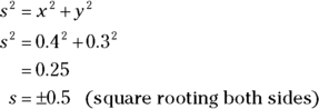
You can reject the negative answer because s obviously has a positive length. So
 .
.Now plug everything into your equation.
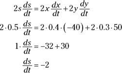
This negative answer means that the distance, s, is decreasing. Thus, when car A is 3 blocks north of the intersection and car B is 4 blocks east of the intersection, the distance between them is decreasing at a rate of 2 mph.
Be sure to differentiate (Step 4) before you plug the given information into the unknowns (Step 5).

FIGURE 7-3: Calculus — it’s a drive in the country.
Filling up a trough
Here’s another garden-variety related rates problem. A trough is being filled up with swill. It’s 10 feet long, and its cross-section is an isosceles triangle with a base of 2 feet and a height of 2 feet 6 inches (with the vertex at the bottom, of course). Swill’s being poured in at a rate of 5 cubic feet per minute. When the depth of the swill is 1 foot 3 inches, how fast is the swill level rising?
1. Draw a diagram, labeling the diagram with any unchanging measurements and assigning variables to any changing things. See Figure 7-4.
Note that Figure 7-4 shows the unchanging dimensions of the trough, 2 feet, 2 feet 6 inches, and 10 feet, and that these dimensions do not have variable names like l for length or h for height. And note that the changing things — the height (or depth) of the swill and the width of the surface of the swill (which gets wider as the swill gets deeper) — have variable names, h for height and b for base (I call it base, not width, because it’s the base of the upside-down triangle shape made by the swill). The swill volume is also changing, so you can call that V, of course.
2. List all given rates and the rate you’re asked to figure out as derivatives with respect to time.
3.a. Write down the formula that connects the variables in the problem: V, h, and b.
Remember the formula for the volume of a right prism (the shape of the swill in the trough)?
Note that this “base” is the base of the prism (the whole triangle at the end of the trough), not the base of the triangle labeled b in Figure 7-4. Also, this “height” is the height of the prism (length of the trough), not the height labeled h in Figure 7-4. Sorry about the confusion. Deal with it.
The area of the triangular base equals ![]() , and the “height” of the prism is 10 feet, so the formula becomes
, and the “height” of the prism is 10 feet, so the formula becomes

This formula contains a variable, b, that you don’t see in your list of derivatives in Step 2. So Step 3 has a second part — getting rid of this extra variable.
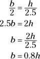
3.b. Find an equation that relates the unwanted variable, b, to some other variable in the problem so you can make a substitution that leaves you with only V and h.
The triangular face of the swill in the trough is similar to the triangular face of the trough itself, so the base and height of these triangles are proportional. (Recall from geometry that similar triangles are triangles of the same shape; their sides are proportional.) Thus,
Similar triangles come up a lot in related rates problems. Look for them whenever the problem involves a triangle, a triangular prism, or a cone shape.
Now substitute 0.8h for b in your formula from Step 3.a.

4. Differentiate this equation with respect to t.
5. Substitute known values for the rate and variable in the equation from Step 4 and then solve.
You know that ![]() cubic feet per minute, and you want to determine
cubic feet per minute, and you want to determine ![]() when h equals 1 foot 3 inches, or 1.25 feet, so plug in 5 and 1.25 and solve for
when h equals 1 foot 3 inches, or 1.25 feet, so plug in 5 and 1.25 and solve for ![]() :
:
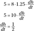
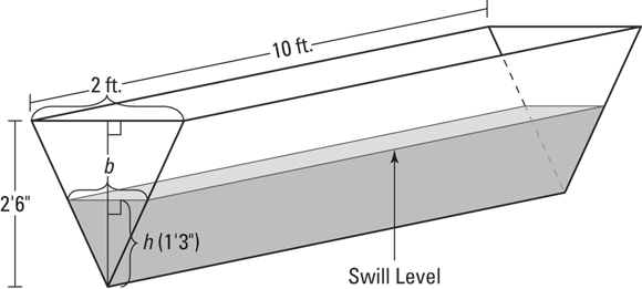
FIGURE 7-4: Filling a trough with swill — lunch time.
That’s it. The swill’s level is rising at a rate of 1/2 foot per minute when the swill is 1 foot 3 inches deep. Dig in.
Linear Approximation
Because ordinary functions are locally linear (straight) — and the further you zoom in on them, the straighter they look — a line tangent to a function is a good approximation of the function near the point of tangency. Figure 7-5 shows the graph of ![]() and a line tangent to the function at the point (9, 3). Near (9, 3), the curve and the tangent line are virtually indistinguishable.
and a line tangent to the function at the point (9, 3). Near (9, 3), the curve and the tangent line are virtually indistinguishable.

FIGURE 7-5: The graph of  and a line tangent to the curve at (9, 3).
Determining the equation of this tangent line is a breeze. You’ve got a point, (9, 3), and the slope is given by the derivative of f at 9:
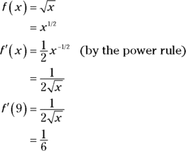
Now just take this slope, ![]() , and the point (9, 3), and plug them into the point-slope form:
, and the point (9, 3), and plug them into the point-slope form:
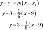
That’s the equation of the line tangent to ![]() at (9, 3). Are you wondering why I wrote the equation as
at (9, 3). Are you wondering why I wrote the equation as ![]() ? It might seem more natural to put the 3 to the right of
? It might seem more natural to put the 3 to the right of ![]() , which, of course, would also be correct. And I could have simplified the equation further, writing it in
, which, of course, would also be correct. And I could have simplified the equation further, writing it in ![]() form. I explain later in this section why I wrote it the way I did.
form. I explain later in this section why I wrote it the way I did.
Now, say you want to approximate the square root of 10. Because 10 is pretty close to 9, and because you can see from Figure 7-5 that ![]() and its tangent line are close to each other at
and its tangent line are close to each other at ![]() , the y-coordinate of the line at
, the y-coordinate of the line at ![]() is a good approximation of the function value at
is a good approximation of the function value at ![]() , namely
, namely ![]() . Just plug 10 into the line equation for your approximation:
. Just plug 10 into the line equation for your approximation:
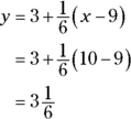
Thus, the square root of 10 is about ![]() . This is only about 0.004 more than the exact answer of 3.1623.
. This is only about 0.004 more than the exact answer of 3.1623.
Now I can explain why I wrote the equation for the tangent line the way I did. This form makes it easier to do the computation and easier to understand what’s going on when you compute an approximation. You know that the line goes through the point (9, 3), right? And you know the slope of the line is ![]() . So, you can start at (9, 3) and go to the right (or left) along the line in the stair-step fashion, as shown in Figure 7-6: over 1, up
. So, you can start at (9, 3) and go to the right (or left) along the line in the stair-step fashion, as shown in Figure 7-6: over 1, up ![]() ; over 1, up
; over 1, up ![]() ; and so on.
; and so on.

FIGURE 7-6: The linear approximation line and several of its points.
So, when you’re doing an approximation, you start at a y-value of 3 and go up ![]() for each 1 you go to the right. Or if you go to the left, you go down
for each 1 you go to the right. Or if you go to the left, you go down ![]() for each 1 you go to the left. When the line equation is written in the above form, the computation of an approximation parallels this stair-step scheme.
for each 1 you go to the left. When the line equation is written in the above form, the computation of an approximation parallels this stair-step scheme.
Figure 7-6 shows the approximate values for the square roots of 7, 8, 10, 11, and 12. Here’s how you come up with these values: To get to 8, for example, from (9, 3), you go 1 to the left, so you go down ![]() to
to ![]() ; or to get to 11 from (9, 3), you go two to the right, so you go up two-sixths to
; or to get to 11 from (9, 3), you go two to the right, so you go up two-sixths to ![]() or
or ![]() . (If you go to the right one half to
. (If you go to the right one half to ![]() , you go up half of a sixth, that’s a twelfth, to
, you go up half of a sixth, that’s a twelfth, to ![]() — the approximate square root of
— the approximate square root of ![]() .)
.)
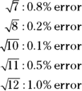
Below are the errors for the approximations shown in Figure 7-6. Note that the errors grow as you get further from the point of tangency (9, 3); also, the errors grow faster going down from (9, 3) than going up from (9, 3) — errors often grow faster in one direction than the other with linear approximations.
Linear Approximation Equation: Here’s the general form for the equation of the tangent line for a linear approximation. The values of a function ![]() can be approximated by the values of the tangent line
can be approximated by the values of the tangent line ![]() near the point of tangency,
near the point of tangency, ![]() , where
, where
This is less complicated than it looks. It’s just the gussied-up calculus version of the point-slope equation of a line you’ve known since Algebra I, ![]() , with the
, with the ![]() moved to the right side:
moved to the right side:
This algebra equation and the above equation for ![]() differ only in the symbols used; the meaning of both equations — term for term — is identical. And notice how both equations resemble the equation of the tangent line in Figure 7-6.
differ only in the symbols used; the meaning of both equations — term for term — is identical. And notice how both equations resemble the equation of the tangent line in Figure 7-6.
Whenever possible, try to see the basic algebra or geometry concepts at the heart of fancy-looking calculus concepts.