12.1 PRICING OF DERIVATIVE CONTRACTS UNDER COLLATERAL AGREEMENTS
The liquidity risk embedded in derivative contracts requires careful analysis because of the complex nature of payoffs and of cash flow profiles. For derivative contracts too the general principle is that the value at inception should be the present value of all future (expected) cash flows, and it should be zero in order to be defined “fair”. All costs and remuneration for risks must be included in the fair value to one of the parties involved,1 hence funding costs and remuneration for liquidity risks have to be considered as well.
Funding costs arise from the replication (i.e., dynamic hedging) strategy of derivative contracts, and in the first part of this chapter we will study how these costs are originated: we will investigate all the components related to funding of the replication strategy and of the collateral accounts in case the contract provides for it.
Currently, most contracts dealt in interbank OTC derivatives are collateralized. A collateral agreement is characterized by the following features, amongst others:
- Initial margin (in some contracts defined as independent amount): This is the amount of cash (or other eligible assets, possibly illiquid) that a counterparty has to post to the other in order to cover potential negative exposure of the derivative contract. It is usually related to as the VaR of the deal and theoretically should be exchanged between parties in a symmetric way.
- Variation margin: This is variation of the collateral subsequent to variation in the NPV of the derivative contract.
- Maintenance margin: This is the level of the collateral below which it is not possible to drop after variation margins are posted. If the balance drops below the level, the initial margin has to be restored.
The most widespread form of collateral agreement is represented by the CSA (i.e., a credit support annex to the ISDA Master Agreement for derivative transactions). Though a legal document, it is not mandatory (banks can in theory sign an ISDA agreement without a CSA), and regulates credit support, represented by collateral, for derivative products.
The CSA defines the asset classes of covered transactions and rules under the terms of which collateral is posted or transferred between derivative counterparties to mitigate credit risk arising from in-the-money derivative positions. If on any valuation date, the delivery amount equals or exceeds the pledgor's minimum transfer amount (MTA), the pledgor is required to transfer eligible collateral with a value at least equal to the delivery amount. The delivery amount is the amount of the CSA that exceeds the value of all posted collateral held by the secured party.
The CSA is equal to the secured party's exposure plus pledgor's independent amount (if any) minus secured party's independent amount (if any) minus the pledgor's threshold.
The collateral to post must meet the eligibility criteria in the agreement (e.g., which currencies it may be in, what types of bonds are allowed, and which haircuts are applied. Rules are defined in order to settle disputes arising over the valuation of derivative positions.
Although a standard CSA is a long way from being defined by practitioners, some market conventions are common features for many CSAs, as there is no threshold or symmetric terms between parties – only cash as eligible collateral is remunerated at the OIS rate.
It is also worthy of note that CSA agreements usually operate on an aggregated basis: the NPVs of all contracts (also for different types of underlying) included in a netting set are summed algebraically and the net amount is posted as collateral by the counterparty who has a negative total NPV. Clauses relating to minimum transfer amount and thresholds also apply. We will not dwell on netting sets, minimum transfer amounts and thresholds in what follows.
Variation and initial margins are commonly remunerated at different rates. The cash posted for variation margin is remunerated at the OIS rate defined for the reference currency, the cash posted for initial margin is typically remunerated at the OIS rate minus. Eligible assets are not remunerated at all and they are typically transferred “free of payment”.
Futures contracts have features similar to CSA agreements, but: the initial margin (collateral) is always required by the clearing house and is determined as a small percentage of the value of future delivery (futures price times the notional of the contract), based on the VaR of the contract. Variation margins occur daily but, differently from the CSA,2 they can be withdrawn if positive to a counterparty, provided that the maintenance margin has not be eroded. In the end they are not real variation margins, but daily liquidation of the variation in terminal value of the contract. There is remuneration for the initial margin, but no remuneration for variation margins.
In what follows we analyse the pricing of derivatives under a CSA agreement, without considering netting, minimum transfer amounts and thresholds. So, we will investigate the pricing of a contract on a “standalone” basis, although we are aware that “incremental” pricing, when netting is considered, may significantly alter the result and then it should not be overlooked if a more refined methodology needs to be applied.
Fujii and Takahashi [70] is a work closely related to the analysis below: they study the effects of imperfect collateralization and introduce a decomposition of total contract value which resembles the one we offer below, which also includes bilateral CVA. On the other hand, we extend their analysis to include the effects that funding costs have on final contract value, disregarding the residual counterparty credit risk due to imperfect collateralization.
Another recent work related to our analysis is [104], which studies the effects of partial collateralization on bilateral credit risk, keeping the costs due to different rates paid and received on the collateral account in mind. Although their pricing fomulae somehow encompass the formulae we give below as well, we believe we offer a different and intuitive approach to the inclusion of funding costs, with the same proviso as before of not considering credit risk. We also have to stress the fact that [104] focuses on deriving a general formula to calculate the price of the contract,3 whereas we try and derive the value of the contract to a counterparty.
12.1.1 Pricing in a simple discrete setting
Let us assume we have an underlying asset S at time 0 that can go up to Su = Su or down to Sd = Sd, with d < 1, u > 1 and u × d = 1 in the next period. Let VC be the price of a contingent claim at time 0 (the “C” at the exponent stands for “collateralized”), and ![]() and
and ![]() its value when the underlying jumps to, respectively, Su and Sd. C is the value of the collateral account to be posted to the counterparty holding a position in the contingent claim when the NPV is positive to it; the collateral account earns collateral rate c. We will assume that percentage γ of the contract's NPV is continuously collateralized, so that at any time C = γV.4 B is the value of a bank account earning risk-free rate r at each period. In this framework, following the classical binomial approach in [56], we build a portfolio of underlying asset S and bank account B perfectly replicating the value of the contingent claim in each of the two states of the world (i.e., possible outcomes of the underlying asset's price), jointly with the value of the collateral account. In other words, we want to replicate a long position in the collateralized contingent claim.
its value when the underlying jumps to, respectively, Su and Sd. C is the value of the collateral account to be posted to the counterparty holding a position in the contingent claim when the NPV is positive to it; the collateral account earns collateral rate c. We will assume that percentage γ of the contract's NPV is continuously collateralized, so that at any time C = γV.4 B is the value of a bank account earning risk-free rate r at each period. In this framework, following the classical binomial approach in [56], we build a portfolio of underlying asset S and bank account B perfectly replicating the value of the contingent claim in each of the two states of the world (i.e., possible outcomes of the underlying asset's price), jointly with the value of the collateral account. In other words, we want to replicate a long position in the collateralized contingent claim.
To do so, we have to set the following equalities in each of the two states of the world:
and
Equation (12.1) states that the value of the contingent claim ![]() , when the underlying jumps to Su from the starting value S, minus the value of the collateral account, must be equal to the value of the replicating portfolio, comprised of α units of the underlying and β units of the bank account. The collateral account at the end of the period will be equal to the initial value C at time 0, plus the interest rate accrued c. The replicating portfolio has to be revalued at prices prevailing at the end of the period (i.e., Su for the underlying asset and initial value B plus accrued interest r for the bank account). In a very similar way, equation (12.2) states that the value of the contingent claim, minus the value of the collateral account, must be equal to the value of the replicating portfolio when the underlying jumps to Sd.
, when the underlying jumps to Su from the starting value S, minus the value of the collateral account, must be equal to the value of the replicating portfolio, comprised of α units of the underlying and β units of the bank account. The collateral account at the end of the period will be equal to the initial value C at time 0, plus the interest rate accrued c. The replicating portfolio has to be revalued at prices prevailing at the end of the period (i.e., Su for the underlying asset and initial value B plus accrued interest r for the bank account). In a very similar way, equation (12.2) states that the value of the contingent claim, minus the value of the collateral account, must be equal to the value of the replicating portfolio when the underlying jumps to Sd.
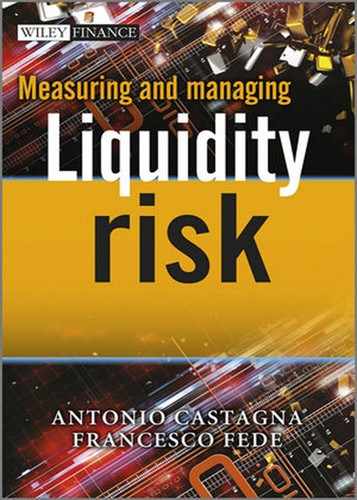
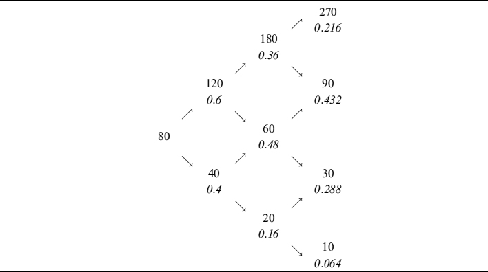
Equations (12.1) and (12.2) can be easily solved for quantities α and β, yielding:
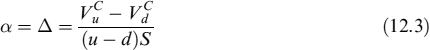
and
We indicated α = Δ because it is easily seen in (12.3) that it is the numerical first derivative of the price of the contingent claim with respect to the underlying asset, as usually indicated in option pricing theory.
If the replicating portfolio is able to mimic payoff of the collateralized contingent claim, then its value at time 0 is also the arbitrage-free price of the collateralized contingent claim:

It is possible to express (12.5) in terms of discounted expected value under the risk-neutral measure and, recalling that C = γVC and rearranging, we get:
with ![]() . The value of the collateralized contingent claim VC is trivially:
. The value of the collateralized contingent claim VC is trivially:
which is the expected risk-neutral value multiplied by the factor ![]() , making the final formula look like the expected value discounted by a rate that is a weighted average of the risk-free and collateral rate, instead of just the risk-free rate, despite the fact we are still in a risk-neutral world.
, making the final formula look like the expected value discounted by a rate that is a weighted average of the risk-free and collateral rate, instead of just the risk-free rate, despite the fact we are still in a risk-neutral world.
The right-hand side of equation (12.6) is also equal to the expression we would get when replicating a contingent claim without any collateral agreement.5 Let VNC be the value of such a claim, then we have:
Equation (12.8) states that a non-collateralized contingent claim is equal to an otherwise identical collateralized claim, minus a quantity we name liquidity value adjustment (LVA) and precisely define as follows.
Definition 12.1.1. LVA is the discounted value of the difference between the risk-free rate and the collateral rate paid (or received) on the collateral over the life of the contract. It is the gain (or loss) produced by liquidation of the NPV of the derivative contract due to the collateralization agreement.
The fact that we are still working in a risk-neutral world is confirmed by the expected return on the underlying asset:
pSu + (1 − p)Sd = (1 + r)S
which is equal to the risk-free rate.
Note that by extending the binomial approach to a multi-period setting, thus introducing a dynamical replicating strategy whereby the contingent claim is replicated by dynamically rebalancing the underlying asset and bond portfolio, the final result of the replica is not terminal payoff of the contingent claim, but includes both the latter and the terminal value of cumulated losses/gains arising from LVA. This has some very important implications at the dealing room level which we examine in Section 13.2.
Example 12.1.1 clarifies how the replication argument works under the collateral and payoff attained at expiry.
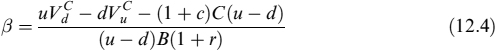
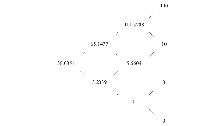
Example 12.1.1. Assume6 we want to price a call option that is fully collateralized (γ = 100%) and written on an underlying asset whose starting value is 80, which is also the strike price. The risk-free rate for one period is r = 0.10, whereas the collateral rate for each period is c = 0:06. The option expires in three periods; at the end of each period the underlying asset can jump upward or downward by a factor, respectively, of u = 1.5 and d = 0.5, so that the probability to jumping upward is p = 0.6. In Table 12.1 we show how the underlying asset price evolves (with the associated probability below each possible outcome).
Table 12.1. Evolution of the underlying asset and (in italics) associated probabilities below each possible outcome
The value of the option can be computed via (12.7) backward recursion starting from the known terminal payoff. The value of the option at each point of the binomial grid is also the value of the collateral account (with the sign reversed). Table 12.2 gives the results and shows the value of the collateralized option at time 0 is VC = 38.0851.
Table 12.2. Value of the call option at each point of the grid and of the collateral account (same but with the sign reversed)
A replicating portfolio can be built be computing the Δ for the underlying asset and the quantity β of the bank account needed to finance the purchase. In Table 12.3 the Δ is shown for each node of the binomial tree along a predefined path of the underlying asset (it is arbitrary and for illustration purposes only); below each Δ we also indicate the quantity to trade in the bank account, plus the interest paid on the amount of the bank account traded in the previous period. At the end of the last period we consider both types of jumps, so as to examine what happens when the option terminates in-the-money or out-of-the-money.
Table 12.3. Amount of underlying asset to trade at each point of the predefined path. Below each Δ the amount of the bank account plus accrued interests from the previous period are shown (in italics)
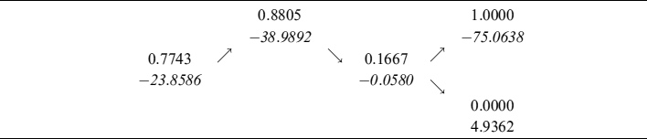
At time 0, the quantity of the underlying to hold in the portfolio to replicate one call option is 0.7743. To finance this purchase, we have to borrow money by selling a bank account for an amount of −23.8586. The difference is the amount of money we have to invest to begin the replication strategy, and it is exactly the value of the option at time 0.
At time 1, Δ = 0.8805 so we have to buy more assets and increase selling the value of the bank account to borrow more money, besides paying accrued interest on the initial borrowing of 23.8586, which we still have. The value of the bank account is then −38.9892. When we arrive at the last period either with one asset in the portfolio or a bank account value of −75.0638, when the option expires in-the-money; otherwise, we end up with no asset or a bank account value of 4.9362 when the option expires out-of-the-money.
There is an additional amount of money to be borrowed when replicating a collateralized option, and this is the amount needed to finance the collateral account value. Hence, a long position in a collateralized option entails a short position in the collateral account, since we have a cash amount of money equal to the value of the contingent claim. The total cost to replicate the collateral account is given by the difference between the risk-free and collateral rate, times the amount of the collateral account at the previous period. In Table 12.4 we show the cost associated to each point of the predefined path we have chosen for the underlying asset; the cost is nil at time 0 and has to be financed for the other periods.
Table 12.4. Cost to replicate the collateral account at each point of the predefined underlying asset's path

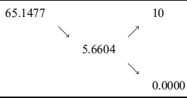
Let us now investigate the replicated value of the call option. This is shown in Table 12.5, where we revaluate at each point of the predefined path the replicating portfolio as far as the quantity of the underlying asset and bank account needed to finance its purchase are concerned. As can easily be seen, the replicating portfolio does not exactly mimic the value of the call, and at expiry the two possible payoffs (i.e., 10 when the call terminates in-the-money and 0 otherwise) do not actually match in either case.
Table 12.5. Replica of the call option with the underlying asset and bank account portfolio

The error in the replica is exactly equal to the cost to finance the collateral account. Actually, when adding the sum of values from Table 12.4 and compounding them at each period with the risk-free rate, we get the total result in Table 12.6, which shows that at each period, including at expiry, the call option value is exactly replicated. At the first period, the total replica is 66.6711 plus the cost of the collateral account 1.5234, for a total of 65.14774, which is exactly the call value in Table 12.2. At the end of the second period, we need to compound 1.5234 at the risk-free rate (0.10) and sum it to the cost for the second period (2.6059). By adding this total cost to the replicated value of the option (9.9420) we finally get the total replication value of 5.6604, once again the same as in Table 12.2. By the same token we can also derive the total replication value at expiry for the two cases of moneyness.
Table 12.6. Call replica including the cost to finance the collateral account
12.1.2 The replicating portfolio in continuous time
Now we extend the binomial approach we sketched above to a continuous and more general setting. Assume the underlying asset follows dynamics of the type:
The underlying has a continuous yield of yt and volatility σt.
The dynamics of the contingent claim are derived via Ito's lemma:
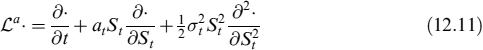
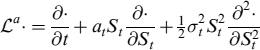
where we used the operator ![]() a· defined as:
a· defined as:
Moreover, we will also set ![]() in what follows. The dynamics of the cash collateral account are defined as
in what follows. The dynamics of the cash collateral account are defined as
where the first part on the left-hand side is variation of collateral dCt = γdVt, equal to fraction γ of variation of the NPV of the contract (the initial value of the collateral account is equal to the collateral C0 = C = γV0); the second part on the left-hand side is the amount of interest produced by the collateral during period dt, given the collateral rate ct. We denote the funding/investment rate by rt. The collateral account can be seen as a bank account (actually, it is a bank account), so that receiving cash collateral means being short the collateral account (such as when shorting a bond and receiving cash). At the end the collateral account (i.e., collateral plus interest) is returned to the transferor (at the same time the final payoff of the contingent claim is received by the transferee).
Remark 12.1.1. It is worth stressing the difference between “collateral” and “collateral account”. Collateral is posted by the party for whom the contract has a negative value, to protect the other party against the risk of default. The collateral account is the sum of collateral received by the party for whom the contract has a positive value, plus the interest it generates, which the receiving party has to pay to the other side.
Evolution of the cash account of a bank is deterministic and equal to:
where, as was the case with the cash collateral account, being short B means receiving cash.
At time 0, the replication portfolio in a long position in derivatives V that is cash-collateralized is set up. It comprises a given quantity of the underlying asset and of the bank account such that their value equals the starting value of the contract and of the collateral:
We have to find a trading strategy {αt, βt} such that it satisfies the following well-known conditions:
- Self-financing condition: No other investment is required to operate the strategy besides the initial one:
- Replicating condition: At any time t the replicating portfolio's value equals the value of the contract and of the collateral:
for t ∈ [0, T].
The way in which the replicating portfolio evolves can be written as:
On the other hand:
Remark 12.1.2. Although evolution of the collateral is equal to fraction γ of the value of contract Vt (i.e., dCt = γdVt), the collateral account Ct also generates an additional cash flow equal to collateral rate ct times collateral amount Ct (i.e., ctCtdt). We added these interest amounts when computing variation of the contract value and of the collateral on the left-hand side of (12.18). We are interested in variation of the collateral account – not simply the collateral – since the strategy needs to replicate the former and not just the latter.
Equating (12.17) and (12.18) and imposing self-financing and replicating conditions, we get:
We can determine α and β such that the stochastic part in (12.19) is cancelled out:
Substituting in (12.19):
Let us split (12.22) in two parts. The first is a standard PDE under the risk-neutral argument:
The second part is more unusual:
It shows how a collateral account evolves under a real world measure by equating the cost of the bank account used to finance it.
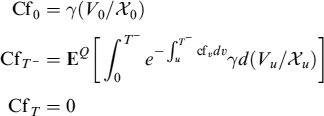
Equation (12.22) has a solution that can be found by means of the Feynman–Kac theorem:
Keeping in mind the fact that the collateral at expiry will be paid back to the counterparty who posted it, CT = 0, we have:
![]()
so that equation (12.25) can be written as:
Equation (12.26) states the same result derived in a binomial setting above: a collateralized claim is equal to the value of an otherwise identical non-collateralized claim, plus the present value of the cost incurred to finance the collateral, or LVA:
![]()
Note that we have not introduced any credit risk until now, so LVA cannot be confused with any adjustment due to the risk of default. On the other hand, it is still possible to derive an arbitrage-free price when the risk-free rate and collateral rate are different, something counterintuitive at first sight.
Recalling that Ct = γVt, equation (12.22) can be equivalently decomposed as:
The solution to (12.27) as a result of applying the Feynman–Kac theorem is:
The second part on the right-hand side is nil, since as before:
We have added the dependency of the value of the claim on the underlying price, whose drift is indicated as superscript characters. Thus, we have perfect analogy with the discrete case examined above.
When the deal is fully collateralized (i.e., γ = 100%), the discount rate in equation (12.29) collapses to collateral rate ct, which is a well-known result (see, amongst others, [69], [89] and [105]). We think equation (12.26) offers more insight. Actually, discounting by means of the collateral rate is a good way of using an effective rate to reproduce the effects of risk-free discounting and LVA. Should we want to disentangle the effects, however, then we should resort to (12.29). For example, in a dealing room correct evaluation of the LVA allows liquidity costs related to collateralization on relevant desks to be correctly allocated. If a collateral desk exists, LVA can be the compensation it receives for managing a given deal, whereas the trading desk closing the deal will be left to manage just the risk-free value of the contract.
12.1.3 Pricing with a funding rate different from the investment rate
Let us assume the operator of the replication strategy is a bank. The difference between the investment and funding rate is due mainly to credit factors (barring the trivial bid/ask factor and liquidity premiums), so that when considering rates actually paid or received by the bank, we should also model default. Nevertheless, this is not necessary since we are assuming that pricing is operated from the bank's perspective.
Actually, the funding rate rF that a bank has to pay, when financing its activity, should just be considered a cost from its own perspective, on the basis of the going concern principle. On the other hand, from the lender's perspective, the spread over the risk-free rate paid by the bank, is the remuneration for bearing the risk of default of the borrowing bank.7
When the bank sells a bank account, it will pay interest rF on received funds until maturity; conversely, when the bank buys a bank account, we assume there is a default risk-free borrower paying risk-free rate r. Evolution of the bank account in (12.13) becomes:
where ![]() and 1{} is an indicator function equal to 1 when the condition at the subscript is verified. If quantity β of the bank account is negative (i.e., the bank borrows money) then the bank account grows at funding rate
and 1{} is an indicator function equal to 1 when the condition at the subscript is verified. If quantity β of the bank account is negative (i.e., the bank borrows money) then the bank account grows at funding rate ![]() ; when quantity β is positive (i.e., the bank lends money) the bank account grows at risk-free rate rt.
; when quantity β is positive (i.e., the bank lends money) the bank account grows at risk-free rate rt.
If a risk-free borrower does not exist such that we actually have to buy bank accounts issued by other defaultable banks, then we can invest at rate rB > r, and the difference between the two rates is remuneration for credit risk. The expected return earned on the investment will be in any case risk-free rate r. Default of the counterparty, to whom the bank lends money, will affect the performance of the replication strategy of the contingent claim in any event, so that counterparty credit risk should be eliminated or mitigated whenever possible. We will come back to this issue later.
Assuming that the funding rate is the risk-free rate plus spread ![]() , we can write the rate at which bank account interest accrues as:
, we can write the rate at which bank account interest accrues as:
Replacing the risk-free rate rt with ![]() in equation (12.22), we get:
in equation (12.22), we get:
From (12.32) we can easily derive two ways to express the value of the contingent claim at time 0 equivalent to formulae (12.26) and (12.29), respectively, as:
and
Equation (12.33) breaks the value of the collateralized contract down as the sum of an otherwise identical non-collateralized deal and of LVA.
To get even more insight and allow for further decomposition useful when allocating revenues and costs within a dealing room, we rewrite equation (12.32) as:
The solution to (12.35) is:
where VNC is the price of a non-collateralized contract assuming no funding spread and LVA is liquidity value adjustment originated by the difference between the collateral and risk-free rate:
and finally FVA is funding value adjustment due to the funding spread and paid to replicate the contract and the collateral account:
where β has been defined above and FVA is a correction to the risk-free value of the non-collateralized contract, which has to be (algebraically) added to the LVA correction. We define it as:
Definition 12..2. FVA is the discounted value of the spread paid by the bank over the risk-free interest rate to finance the net amount of cash needed for the collateral account and the underlying asset position in the dynamic replication strategy.
It is interesting to break total FVA down into its components: this decomposition is not essential as far as pricing is concerned, but it is very useful within a dealing room to charge the desks involved in trading (we will dwell more on this later). Let us now isolate the initial part of total FVA due to the funding cost of the replication strategy of the premium and the collateral:
and the second part relating to the funding cost borne to carry the position of the underlying asset in the replication strategy:
Hence, total funding value adjustment is FVA = FVAP + FVAU. Since the indicator function 1{β<0} appears in both components, the FVA of individual components takes the net funding need into account at the financial institution level. Thus, single trading desks also enjoy funding benefit at an aggregated level.
For example, consider the FVA for the cost borne to fund the underlying asset's position: the derivatives desk should pay the funding costs when it has a positive position, but this cost is paid only if the net amount of the bank account is negative (β < 0). When the underlying asset's position is positive but the net amount in the bank account is positive (β > 0), the derivatives desk will not be charged for any funding cost, although it actually requires funds to buy the asset.
We are now in a position to analyse five different cases:
- Let us assume we have to replicate a contingent claim that has a constant positive-sign NPV (e.g., a long European call option) with a constant positive-sign Δt. Since Vt − Ct − ΔSt is always negative (implying borrowing), the total amount of bank account β is always negative, implying that we always have to borrow money in the replica at rate rF. The pricing equation (12.35) then reads:
Although the decomposition in (12.36) still applies, pricing can be performed very simply by means of an effective discount rate:
So we can simply replace the risk-free rate with the funding rate paid by the bank and perform the same pricing as when lending and borrowing rates are equal. Equation (12.42) is a very convenient way of computing the price at 0 of the contracts, but is of little use in allocating its components to the different desks of the bank.
- When the same (as in point 1) contingent claim (constant positive-sign NPV and Δ) is short, the underlying asset has to be sold in the replication strategy as well, which implies that β > 0 and that the bank always has to invest at the risk-free rate. The pricing formula will be as in formula (12.26) (with reversed signs since we are selling the contract). In this case FVA will be nil. An example of this claim is a short European call option.
- Let us now assume that the contingent claim has a constant positive-sign NPV, but its replication implies a negative position in the underlying asset (e.g., a long European put option), then once again we have β > 0 at any time. The pricing formula is (12.26) in this case too (i.e., the same as in the case with no funding spread).
- If the NPV has a constant negative sign and the replica entails a long position in the underlying (e.g., short European put option), then the total amount of bank account β is always negative, implying that we always have to borrow money in the replica at rate rf. The pricing formula is (12.42) (as in point 1).
- Finally, if the NPV has a constant positive or negative sign and the Δ can flip from one sign to the other, then it is not possible to determine the sign of amount β of the bank account throughout the entire life of the contract. In this case the pricing formula (12.35) cannot be reduced to a convenient representation as in the cases above, and very likely has to be computed numerically. Examples of contracts with non-constant sign Δ are exotic options, such as reverse knockouts.
From the analysis above it is also clear that when the contract is fully collateralized, the effective discount rate is just the collateral rate, whereas the drift rate of the asset can be either the risk-free rate or the funding rate depending on whether the bank account always preserves, respectively, a positive or negative sign until expiry.
Example 12.1.2. We now show a simple example of how these ideas can be put into practice for a European call option on an underlying asset that could be an equity, an FX spot rate or a commodity. Typically, the model used to price options in these cases is the standard Black and Scholes one:
where N() is the normal cumulated distribution function, F = Se(r−y)T is the forward price and:
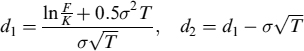
Equation (12.43) valuates a call expiring at T, struck at K, when the underlying spot price is S.
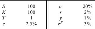
Assume we want to price the call option with the input data in Table 12.7. Since a European call option is a contract of the type shown in point 1 of our list, decomposition of the total value into the several components can be done withut computing the integral in the definition of LVA and FVA.
Actually, the risk-free non-collateralized value of the call (with risk-free rate drift to set the forward price) can immediately be computed as:
VNC = VNC−RF−RD = C(S, K, T, σ, r, y, r)
Table 12.7. Input data for a European call option
The total adjustment of a collateralized option, keeping in mind funding costs both in the discounting and in the drift of the asset to set the forward price, is:
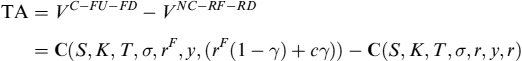
Superscript C/NC stands for collateralized/non-collateralized, RF/FU for risk-free/funding rate discounting and RD/FD for risk-free/funding rate drift.
The quantity TA can be decomposed as follows:
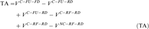
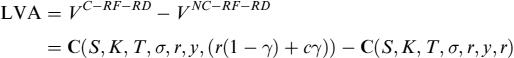
Now, LVA is represented by the third line of equation (TA) and can be computed by the Black and Scholes formula:

Total FVA is represented by the first two lines of equation (TA); namely, the difference between the collateralized option, discounted by the funding rate and drift equal to the funding rate, and the non-collateralized option, discounted by the risk-free rate and drift equal to the risk-free rate:
FVA = VC−FU−FD − VC−RF−RD
We can break total FVA down by recognizing that FVAU (i.e., FVA due to the underlying asset) is the difference in the first line of equation (TA):

FVA due to the premium and collateral is:

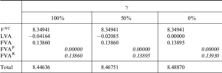
In Table 12.8 we show decomposition of the total option value into the components examined for different percentages γ of collateralization of the contract's NPV. It is quite obvious that for the non-collateralized contract (γ = 0%) LVA is nil. Note also that the total values can be computed straightforwardly via formula (12.42), clearly obtaining the same result. Nevertheless, with this slightly longer procedure we are able to exactly disentangle the different cost contributions.
Table 12.8. Decomposition of the call option value into the risk-free, LVA and FVA components
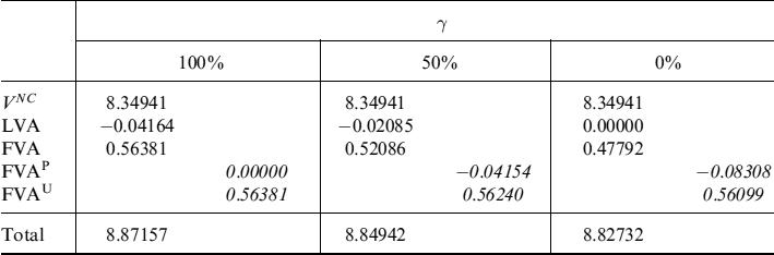
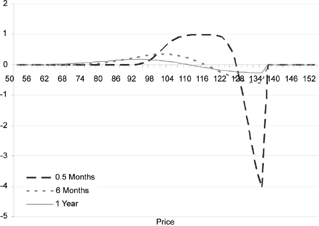
Figure 12.1. Delta of an up-and-out call option with different times to maturities as a function of the price of the underlying asset. The barrier is at 135 and all other data are as in Example 12.1.2
Example 12.1.3. Let us now assume we have the same data as in Example 12.1.2 and that the European call is no more plain vanilla, but has a barrier set above the strike level at 135. The option is an up-and-out call and can be priced in a closed-form formula in a Black and Scholes economy (see [44] for a thorough discussion of barrier options and for pricing formulae, with a focus on the FX market).
In this case it is not possible to use the decomposition used in Example 12.1.2 because the Δ of the up-and-out call can flip from one sign to the other, depending on the level of the underlying asset. We are now in the fifth case of the above list. In Figure 12.1 we depict the Δ as a function of the price of the underlying asset, for three different times to maturity, progressively approaching the contract's expiry: the plots simply confirm what we have written. In this case we resort to a numerical integration of formulae (12.37) and (12.38).8
Table 12.9. Decomposition of the value of an up-and-out call option in its non-collateralized risk-free value, LVA and FVA
Decomposition of the price is given in Table 12.9 only for the case when the contract if fully collateralized (γ = 100%). This means that FVA contains only the component related to financing of the underlying asset. The lower amount of both LVA and FVA with respect to the corresponding European plain vanilla call just examined is easily justified.
12.1.4 Funding rate different from investment rate and repo rate
We now introduce the possibility of lending and borrowing money (or, alternatively, the underlying asset) via a repo transaction. This is actually the way traders finance and buy the underlying asset (typically in the stock market), by borrowing money and lending the asset as collateral until expiry of the contract.
A repo transaction can be seen as a collateralized loan and the rate paid is lower than the unsecured funding rate of the bank, since in case of default of the borrower, the asset can be sold to guarantee the (possibly only partial) recovery of the lent sum. The difference between repo rate rE and the risk-free rate is due to the fact that the underlying asset can be worth less than the lent amount when default occurs: so volatility of the asset and probability of default both affect the repo rate.
We assume that the repo rate is the same when borrowing money or lending money against the underlying asset (repo and reverse repo). This means that we are assuming that the two banks involved in the transaction have the same probability of default with the same recovery rate in the event of default. We will investigate replication costs and the pricing formulae for four of the five possible cases in the list above.
A repo transaction is the proper way to finance buying the underlying asset in the replication strategy. On the other hand, if we really want to consider the actual alternatives that are available to a trader to invest received sums in a less credit-risky way, reverse repo seems an effective option in most cases. So, as far as the buying and selling of the underlying asset are concerned, we go back to the case when there is no asymmetry between investment (lending) and the funding rate, although the risk-free rate is replaced by the repo rate. The amount to be lent/borrowed via the bank account is now:
whereas the quantity αt = Δt of the underlying asset is repoed/reverse-repoed, thus paying/receiving interest ![]() . Replacing these quantities in equation (12.22), we get:
. Replacing these quantities in equation (12.22), we get:
The solution to (12.45) is:
where, as usual, VNC is the price of the non-collateralized contract assuming no funding spread and repo, LVA is liquidity value adjustment due to the collateral agreement:
![]()
and FVA is funding value adjustment:
FVA in this case is split into the funding cost needed to finance the collateral ![]() and the spread of the repo rate over the risk-free rate
and the spread of the repo rate over the risk-free rate ![]() paid on the position of amount Δt of the underlying asset.
paid on the position of amount Δt of the underlying asset.
To better understand how total FVA is built, we split formula (12.47) into two components: the first is FVAP, the cost borne to fund the premium and the collateral (it is the same as in (12.39)). The second part refers to the repo cost to buy or sell the underlying asset to replicate the payoff:
Furthermore, it is possible in this case to rewrite (12.46) in a more convenient fashion for computational purposes:
Formula (12.49) applies to the five cases analysed in the previous section: the discount factor depends on the sign of the bank account needed to fund the collateral account, whereas the drift of the underlying asset is always the repo rate rE.
Example 12.1.4. We revert to Example 12.1.2 for the pricing of a European call option, but we now assume that the bank can buy or sell the underlying asset via repo transactions. We ascertain how the components of total value change in this case. We still use the same inputs as in Table 12.7, but we add to them the repo rate set at rE = 2.25%, which is lower than the unsecured funding rate rF = 3%, but higher than the risk-free rate r = 2% to account for volatility of the collateral (the underlying asset) and the possibility of a smaller collateral value on default of the borrower (the bank).
Let us exploit once again the fact that a European option is a type of contract that falls in the first case analysed above and keep the same considerations we made in Section 12.1.2.
Table 12.10. Decomposition of the value of the call option into the risk-free, LVA and FVA components when the underlying asset is traded via repo contracts
We define LVA as above:
and the two components of FVA as:

Decomposition of total option value into the different components for different percentages of collateralization is given in Table 12.10.
12.1.5 Interest rate derivatives
As far as the pricing of interest rate derivatives is concerned, we have to consider the credit issue as being critically important. Despite analysing replication of a contingent contract with repo transactions, which virtually eliminates credit risk, or at least makes it negligible, unfortunately, it is not possible to replicate interest rate derivatives with such a low level of credit risk, since the replication strategy involves unsecured lending (besides the borrowing) as part of the underlying itself. For example, without credit risk, a FRA can be replicated by selling/buying a shorter maturity bond and buying/selling a longer maturity bond. With credit risk this strategy is clearly flawed since the counterparty to whom we lent money can default before expiry of the bond.
This means that in practice basic interest rate derivatives are no longer real derivatives, but primary securities that cannot be replicated by means of other primary securities (e.g., bonds). The derivative contract can be made credit risk-free by a collateral agreement, but we can no longer set up a strategy to replicate the payoff and evolution of the collateral account, as we have done above for derivatives on different assets. The implications of being unable to implement a replication strategy become apparent by analysing a couple of contracts: a forward rate agreement (FRA) and an interest rate swap (IRS).
Forward rate agreement
Let us introduce a setup to price interest rate derivatives under collateral agreements.9 Let us consider times t, Ti−1 and Ti, t ≤ Ti−1 < Ti. The time t forward rate is defined as the rate to be exchanged at time Ti for the Libor rate Li(Ti−1) = L(Ti−1, Ti) fixed at time Ti−1, in a FRA(t; Ti−1, Ti) contract, so that the contract has zero value at time t.
In the absence of credit risk (i.e., in a single-curve environment), the forward rate can be determined via a portfolio of long and short zero-coupon bonds. The absence of arbitrage also implies the existence of a single, risk-free, discounting curve. Let us assume we have a discount curve denoted by D; we then have:
The FRA fair forward rate can be set according to definition of the contract:
Let us now assume we are in a credit-risky economy. Selling and buying bonds does not allow replicating the FRA payoff since it is always possible that the counterparty to whom we lent money defaults. The forward that is being traded in the market in this case should be simply considered as the expected value of Libor at the fixing time. If we accept that market quotes refer to trades between counterparties with a collateral agreement, then we can quite safely assume that the expected value is taken under a risk-free bond numeraire. The pricing formula is similar to the one presented above for contracts on other underlying assets, although in this case it is not derived from a replication argument, rather it is an assertion:
that is, the expected Libor rate under the Ti forward measure of the value of the contract at expiry Ti−1 plus LVA. In (12.52) Ti = Ti − Ti−1.
The LVA in this case is the present value of the difference between the risk-free rate ![]() and the collateral rate Oj(t), fixed at date tj−1 and valid until date tj, applied to fraction γ of the value of contract FRA(tj; Ti−1, T2) for a total of N days between t and the forward settlement T1, so that tN = T1:
and the collateral rate Oj(t), fixed at date tj−1 and valid until date tj, applied to fraction γ of the value of contract FRA(tj; Ti−1, T2) for a total of N days between t and the forward settlement T1, so that tN = T1:

where ![]() is the difference in the fraction into which the year is split between two rebalancing times of the collateral: one day in our case. Formula (12.52), given the definition of LVA in (12.53), is recursive. We assume that market quotes for FRAs refer to the case when LVA is nil. This means that the collateral rate is supposed to be risk-free rate LD(t; tj−1, tj) = O(t; tj−1, tj), for all j, which is not unreasonable since standard CSA agreements between banks provide for remuneration of the collateral account at the OIS (or equivalent for other currencies) rate. The OIS rate can also be considered as a virtually risk-free rate or at least as embedding a negligible spread for default risk. If this holds true, then equation (12.52) reads as:
is the difference in the fraction into which the year is split between two rebalancing times of the collateral: one day in our case. Formula (12.52), given the definition of LVA in (12.53), is recursive. We assume that market quotes for FRAs refer to the case when LVA is nil. This means that the collateral rate is supposed to be risk-free rate LD(t; tj−1, tj) = O(t; tj−1, tj), for all j, which is not unreasonable since standard CSA agreements between banks provide for remuneration of the collateral account at the OIS (or equivalent for other currencies) rate. The OIS rate can also be considered as a virtually risk-free rate or at least as embedding a negligible spread for default risk. If this holds true, then equation (12.52) reads as:
so that we retrieve the standard result, as in [89], that the FRA fair rate is the expected value of Libor at the settlement date of the contract under the Ti forward risk measure at expiry:
Despite assuming that the market FRA settles at Ti, according to market conventions it actually settles the present value of the Ti payoff at Ti−1. The market FRA fair rate is then different from the “theoretical” rate in (12.55), since the latter should be corrected by means of convexity adjustment as discussed in [91]. The adjustment is nevertheless quite small (fraction of a basis point) and can be neglected under typical market conditions, so we will not consider it.
When the collateral agreement provides for remuneration of the collateral that is different from the OIS rate, then we have LVA ≠ 0, and the FRA fair rate has to be valued recursively. Let ![]() be the spread between the daily risk-free rate and the collateral rate and assume it is a stochastic process independent of the value of the FRA; we can rewrite equation (12.53) as:
be the spread between the daily risk-free rate and the collateral rate and assume it is a stochastic process independent of the value of the FRA; we can rewrite equation (12.53) as:

The second expectation in (12.56) is ![]() , so that we finally get:
, so that we finally get:

In much the same way, we can derive the FVA for an FRA: let ![]() be the funding rate paid by the bank (same notation as above). When financing the collateral (i.e., when the NPV of the contract is negative to the bank), it has to pay this rate to fund the collateral it has to post. In the opposite situation (i.e., when the NPV is positive), the bank invests the collateral received at the risk-free rate, paying the collateral rate.
be the funding rate paid by the bank (same notation as above). When financing the collateral (i.e., when the NPV of the contract is negative to the bank), it has to pay this rate to fund the collateral it has to post. In the opposite situation (i.e., when the NPV is positive), the bank invests the collateral received at the risk-free rate, paying the collateral rate.
Let ![]() be the funding spread over the risk-free rate and assume it is not correlated with the NPV of the FRA. FVA is then:
be the funding spread over the risk-free rate and assume it is not correlated with the NPV of the FRA. FVA is then:

where E[X−] = E[min(X, 0 )]. It is easy to check that:

where Floorlet(tj; Ti−1, Ti, K) is the price of a floorlet at time tj, expiry at Ti−1, settlement at Ti, with strike K. If the bank has a short position in the FRA, then FVA is

where Caplet(ti; Ti−1, Ti, K) is the price of a caplet and the arguments of the function are the same as for the floorlet.
The total value of the FRA is:

In any case, the fair rate making the value of the contract at inception zero, has to be computed recursively.
Interest rate swap
Let us now consider an IRS whose fixed leg pays a rate denoted by K on dates ![]() . The present value of these payments is obtained by discounting them with discount curve D. The floating leg receives Libor fixings on dates Ta, …, Tb and the present value is also obtained by discounting with discount curve D. We assume that the set of floating rate dates includes the set of fixed rate dates. The value at time t of the IRS is:
. The present value of these payments is obtained by discounting them with discount curve D. The floating leg receives Libor fixings on dates Ta, …, Tb and the present value is also obtained by discounting with discount curve D. We assume that the set of floating rate dates includes the set of fixed rate dates. The value at time t of the IRS is:
where LVA is defined as:

where ![]() . LVA in this case is once again the difference between the risk-free rate and the collateral rate applied to fraction γ of the NPV, for a total of N days occurring between valuation date t and the end of the contract tN = Tb.
. LVA in this case is once again the difference between the risk-free rate and the collateral rate applied to fraction γ of the NPV, for a total of N days occurring between valuation date t and the end of the contract tN = Tb.
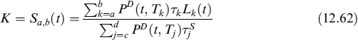
As far as swaps are concerned, we make the assumption that market quotes refer to the situation when LVA = 0, implying that the risk-free and collateral rates are the same. The market swap rate is then the level making the value of the contract at inception Ta zero:
When the risk-free and collateral rates are different, LVA can be evaluated in much the same was as the FRA. We then have:

The second expectation in (12.63) is ![]() , where Ea,b is the expectation taken under the swap measure, with the numeraire equal to annuity
, where Ea,b is the expectation taken under the swap measure, with the numeraire equal to annuity ![]() . So we can finally write:
. So we can finally write:

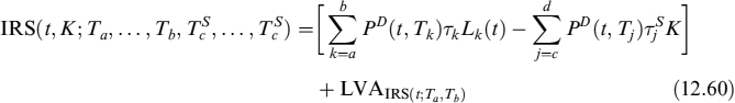
FVA can also be defined analogously with the FRA case and, using the same notation as above, we have:

We can make use of the option on swaps to express the second expectation in (12.65) as:
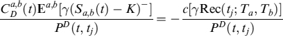
where Rec(t; Ta, Tb) is the price of a receiver swaption priced at time tj, expiry at Ta, on a swap starting at Ta and maturing at Tb, with strike K. If the bank has a short position in the IRS (i.e., it is a fixed rate receiver), then FVA is
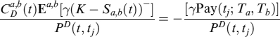
where Pay(t; Ta, Tb) is the price of a payer swaption and the arguments of the function are the same as for the receiver.
Finally, the total value of IRS is:
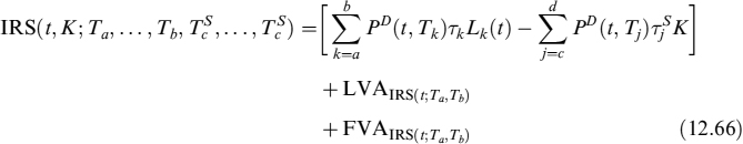
At inception, the swap rate K = Sa,b(t) is the level that makes the value of the contract zero, which can be computed recursively from (12.66).10
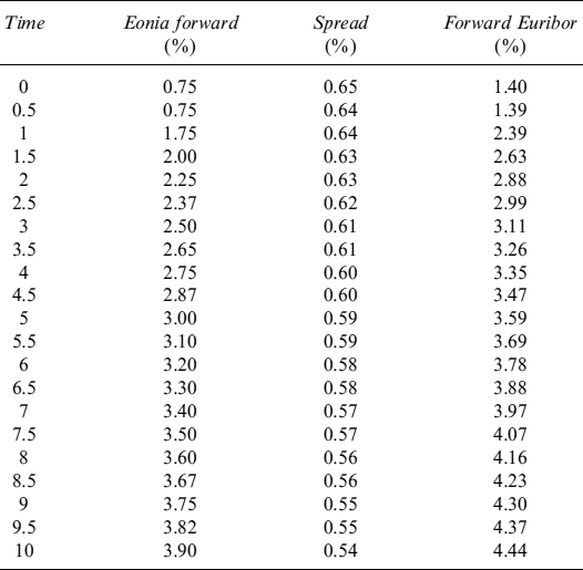
Example 12.1.5. Let us consider an IRS, assuming the risk-free rate is equal to the Eonia rate and Euribor forward fixings are at spreads over the Eonia rate. Yearly Eonia forward rates, spreads and Euribor forward rates are shown in Table 12.11.
Table 12.11. Yearly OIS forward rates and spreads over them for forward Euribor fixings
We price, under a CSA agreement with full collateralization (γ = 100%), a receiver swap whereby the bank pays the Euribor fixing semiannually (set at the previous payment date) and receives the fixed rate annually. Keeping market data in mind, the fair rate can easily be calculated by formula (12.62) and found to be equal to 3.3020. We also assume that the bank has to pay a funding spread of ![]() over the Eonia curve. Finally, we assume that collateral is remunerated at the Eonia rate.
over the Eonia curve. Finally, we assume that collateral is remunerated at the Eonia rate.
Under these assumptions, the LVA of the swap is nil, as is clear from its definition in (12.64). FVA is different from zero, since there is a funding spread. To compute the FVA in (12.65), we have to compute a portfolio of payer swaptions. To this end we make a simplifying assumption that the NPV of swaptions is constant between two Euribor fixing dates (i.e., it is constant over periods of six months). Swaptions can be computed by means of volatilities in Table 12.12 using a standard Black formula. It is then possible to plot the profile of the NPVs of swaptions, which is actually the (approximated) expected negative exposure (ENE) of the receiver swap (the profile is plotted in Figure 12.2).
The results are given in Table 12.13. FVA is quite small for a swap starting at-the-money, accounting for about half a basis point: an almost negligible impact on the fair swap rate including the funding costs. This rate should be set by a numerical search and is the rate making the value of the swap zero, given by the risk-free component plus FVA at inception.
A more conservative FVA can be based on potential future exposure (PFE) rather than expected exposure as we did with ENE. PFE is computed in much the same way as ENE, but considering the level of the future swap rate set at a given confidence level instead of the forward level. We choose 99% as the confidence level.11 PFE is plotted in Figure 12.3 and the results are shown in Table 12.14. In this case, FVA is larger as a percentage of the notional and accounts for about 7 bps when included in the fair rate.
Table 12.12. Implied volatilities for the portfolio of swaptions used to replicate the ENE of the receiver swap
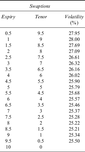
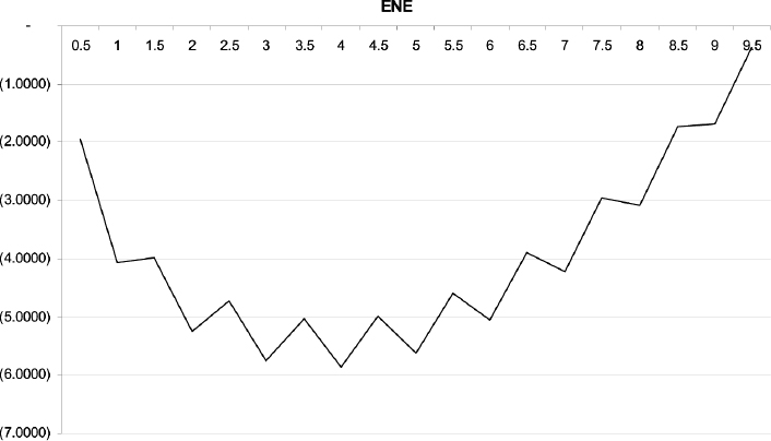
Figure 12.2. ENE of the receiver swap
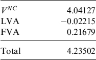
Table 12.13. Fair swap rate, FVA and FVA-adjusted fair swap rate
| FVA | −0.0512% |
| Fair swap rate | 3.3020% |
| Swap rate including FVA | 3.3079% |
| Difference | 0.0059% |
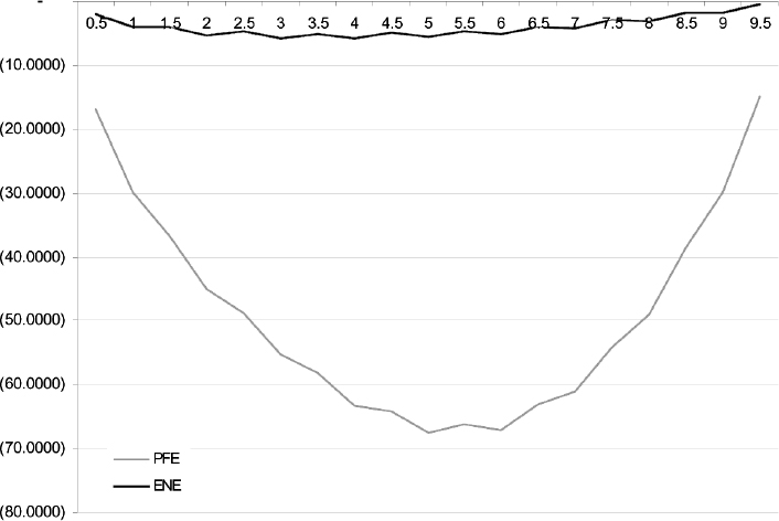
Figure 12.3. PFE of the receiver swap
Table 12.14. Fair swap rate, FVA and FVA-adjusted fair swap rate using PFE
| FVA | −0.6265% |
| Fair swap rate | 3.3020% |
| Swap rate + collateral fund | 3.3728% |
| Difference | 0.0708% |
FVA is rather small when the swap starts and is at-the-money. It can become bigger and bigger as the NPV of the swaps evolves and becomes more negative, or it can become completely negligible as NPV increases.
12.2 PRICING OF COLLATERALIZED DERIVATIVE CONTRACTS WHEN MORE THAN ONE CURRENCY IS INVOLVED
In this section we complete the analysis conducted in Section 12.1 by investigating the valuation of collateralized derivative contracts when more than one currency is involved. This can happen for three reasons:
- The contract payoff is denominated in some currency YYY but collateral is posted in another currency XXX.
- The contract is written on an FX rate.
- The contract payoff depends on assets or market variables denominated in different currencies (e.g., a cross-currency interest rate swap).
In theory, many currencies could be involved, but in what follows we restrict our analysis to when only two currencies have to be considered. We analyse all the cases enumerated above and define liquidity value adjustments and funding value adjustments for collateralized contracts.
12.2.1 Contracts collateralized in a currency other than the payoff currency
Let us assume we have to value a contract whose underlying asset follows dynamics of type:
dSt = (µt − yt)Stdt + σtStdZt
The underlying has a continuous yield of yt and volatility σt and is denominated in a currency that we name “domestic” and refer to as YYY. There is also a foreign currency XXX and an exchange rate X = XXXYYY12 following the dynamics:
dXt = ηtXtdt + vtXtdWt
with dWtdZt = ρdt.
We want to replicate a derivative contract V written on S, which is collateralized continuously in XXX instead of YYY; the latter would normally be the case. Following the same approach outlined in Section 12.1, we build a portfolio replicating both the underlying and the collateral account.
The dynamics of the contingent claim are derived via Ito's lemma:
![]()
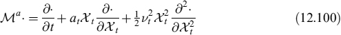
where we used operator ![]() a· defined as:
a· defined as:
Moreover, we will set ![]() in what follows. The dynamics of the cash collateral account are defined as
in what follows. The dynamics of the cash collateral account are defined as
![]()
The account is denominated in XXX as long as it earns the collateral rate cft; rft is the funding/investment rate in YYY. For the collateral account it is also true that:
Evolution of the YYY bank cash account is deterministic and equal to:
and evolution of the XXX bank cash account is:
At time 0, the replication portfolio in a long position in derivative V, YYY cash-collateralized, is set up with a given quantity of the underlying asset and of XXX and YYY bank accounts such that their value equals the starting value of the contract and of the collateral account:
As usual, we impose self-financing and replicating conditions to find quantities {αt, βt, θ}. We can write the way in which the replicating portfolio evolves as:
On the other hand:
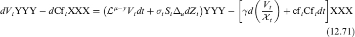
Equating (12.70) and (12.71) we get:
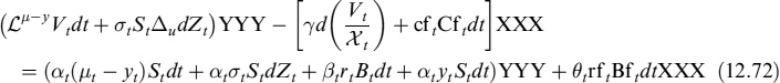
We can determine α and β such that the stochastic part in (12.72) is cancelled out:
Substituting in (12.72):
We can express equation (12.74) in terms of YYY only by multiplying the second term by FX rate Xt and then we have:
where C is the collateral account converted in YYY units (we suppressed indication of the currency to lighten the notation).
It can be shown (see Section 12.1) that the solution to equation (12.75) is:
which is the same result as when the collateral is posted in YYY, with the only difference that the amount of the collateral account in YYY is multiplied by the difference between the risk-free rate and the collateral rate applied to the collateral amount in XXX units.
We can also denote the second part of the formula as the LVA, which is the present value of the cost incurred to finance the collateral in XXX units:
![]()
Recalling that Cft = γ(Vt/Xt)XXX, or Ct = γVtYYY, equation (12.75) has another solution:
In this equation we added the dependency of the value of the claim on the underlying price, whose drift is indicated by superscripts. In practice, we can use standard valuation formulae derived, for example, in a Black and Scholes economy by simply changing the discount rate: this will no longer be the only domestic YYY risk-free rate, there will also be a correction depending on collateralization percentage γ and on the foreign XXX risk-free and collateral rates.13
Remark 12.2.1. The value of a contract, collateralized in a currency different from the one in which the payoff is denominated, does not depend on the FX rate X, but on the risk-free and collateral rates of currency XXX, in addition to the risk-free rate of currency YYY.
Pricing with funding rate different from investment rate
Let us assume that the replication strategy is operated by an agent (say, a bank), for which the investment and funding rates are different, due mainly to credit factors. The bank pays funding rate rF when financing its activity in the domestic YYY currency; analogously, rfF is the rate that it pays when financing its activity in the foreign YYY currency. Evolution of the domestic bank account in (12.67) is:
where ![]() and 1{} is the indicator function equal to 1 when the condition at the subscript is fulfilled. The XXX bank account evolves as follows:
and 1{} is the indicator function equal to 1 when the condition at the subscript is fulfilled. The XXX bank account evolves as follows:
The funding rate can be written as the risk-free rate plus a spread:
and similarly for the foreign rate
Replacing risk-free rates rt and rft with ![]() and
and ![]() in equation (12.75), we get:
in equation (12.75), we get:
From (12.82) we can easily derive the two ways of expressing the value of the contingent claim at time 0 equivalent to formulae (12.76) and (12.77), respectively, as:
and
In equation (12.83) decomposition of the collateralized contract value is given as the sum of the otherwise identical non-collateralized deal and of LVA.
We would also like to isolate the effect due to the funding spread, so we introduce a further decomposition by rewriting equation (12.82) as:

The solution to (12.85) is:
where VNC is the price of the non-collateralized contract assuming no funding spread, LVA is the liquidity value adjustment originated by the difference between the collateral and risk-free rate:
and, finally, FVA is the funding value adjustment due to the funding spread, which is paid to replicate the contract and the collateral account:
where β is defined as above. FVA is the correction to the risk-free value of the non-collateralized contract that has to be (algebraically) added to the LVA correction. For a definition of LVA and FVA see [45].
We are now in a position to analyse five different cases:
- Let us assume a contingent claim with a constant positive-sign NPV (e.g., a long European call option) with a constant positive-sign Δt has to be replicated. In this case βt = Vt − ΔSt < 0 and θt = −Ct < 0 always (implying borrowing always takes place in both currencies). The pricing equation (12.85) then reads:
Although the decomposition in (12.86) still applies, pricing can be performed very simply by means of an effective discount rate:
So we can simply replace the risk-free rate with the funding rate paid by the bank and perform the same pricing as when lending and borrowing rates are the same.
- When the same contingent claim (constant positive-sign NPV and Δ) as in point 1 is sold, the underlying asset has also to be sold in the replication strategy, which implies that βt > 0 and that the bank always has to invest at the risk-free rate in YYY; the bank account in XXX, θt = −Ct, will always be positive as well. The pricing formula will be the same as in formula (12.77) (with reversed signs since we are selling the contract). In this case FVA will be nil. An example of this claim is a short European call option.
- Let us now assume that the contingent claim has a constant positive-sign NPV, but its replication implies a negative position in the underlying asset (e.g., a long European put option). So, once again we not only always have βt = Vt − ΔSt0 > 0, but also θt = −Ct < 0, implying that the bank has to borrow money in XXX. PDE (12.85) now reads:
Pricing can be performed via the compact formula:
In this case we replace the risk-free rate with the funding rate paid by the bank for XXX.
- If the NPV has a constant negative sign and the replica entails a long position in the underlying (e.g., short European put option), then the total amount of bank account βt = Vt − ΔSt < 0 is always negative, implying that the bank always has to borrow money in the replica at rate rF in YYY; since θt = −Ct > 0 always, the bank will invest the collateral at the risk-free rate rf. The pricing formula is derived similarly to (12.92) and is:
- Finally, if the NPV has a constant positive or negative sign and the Δ can flip from one sign to the other, then it is not possible to determine the sign of amount βt of the bank account throughout the entire life of the contract, although it is always possible to determine whether θt is always positive or negative. In this case pricing formula (12.85) cannot be reduced to a convenient representation as in the cases above and has to be done so numerically.
Funding rate different from investment rate and repo rate
We mentioned in Section 12.1 that the proper way to finance buying of the underlying asset in the replication strategy is through a repo transaction. On the other hand, if we really want to consider the actual alternatives available to a trader to invest received sums in a less credit-risky way, reverse repo seems an effective option in most cases. The amount to be lent/borrowed via domestic and foreign bank accounts is now:
where quantity αt = Δt of the underlying asset is repoed/reverse-repoed, thus paying/receiving interest ![]() . Replacing these quantities in equation (12.75), we get:
. Replacing these quantities in equation (12.75), we get:
The solution to (12.94) is:
where, as usual, VNC is the price of the non-collateralized contract assuming no funding spread or repo, LVA is the liquidity value adjustment due to the collateral agreement:
![]()
and FVA is the funding value adjustment:
FVA is split into the funding cost needed to finance collateral ![]() and the spread of the repo rate over the risk-free rate
and the spread of the repo rate over the risk-free rate ![]() paid on the position of amount Δt of the underlying asset in this case.
paid on the position of amount Δt of the underlying asset in this case.
To better understand how total FVA is built, we split formula (12.96) into two components: the first is FVAP, the cost borne to fund the premium and the collateral, and is the same as in (12.88). The second part refers to the repo cost to buy or sell the underlying asset to replicate the payoff:
Furthermore, in this case it is possible to rewrite (12.95) in a more convenient fashion for computational purposes:
Formula (12.98) is applicable to the five cases analysed in the previous section: the discount factor depends on the sign of the bank account needed to fund the collateral account, whereas the drift of the underlying asset is always repo rate rE.
12.2.2 FX derivatives
We now want to compute the value to the bank of an FX derivative contract: it is a function of FX rate X and of time V(Xt, t). We start with a simple forward contract, named outright in the FX market.
Collateral posted in numeraire currency
When collateral is posted in numeraire currency YYY, the case examined in Section 12.1 for a general derivative contract is applicable, although here we need to replace the underlining asset with the exchange rate. We focus only on the more realistic case of different borrowing/lending rates and apply the replication argument as before.
The difference between FX trades and trades in other securities (say, equities) is that, in the case of FX, we are actually buying money in some currency by paying a price in another currency, and money received can be invested in a bank account that we assume to be default risk free.14 So by buying, for example, foreign currency XXX (which we assumed to be the base), the bank can invest this amount in a XXX-denominated bank account. On the other hand, when the bank needs to short the base currency to buy numeraire currency, it has to borrow money in XXX.
The evolution of contract V(Xt, t) = Vt, according to Ito's lemma, is:
where
The replicating portfolio comprises at time t a given amount αt of the base currency XXX worth Xt and a given amount of cash βt borrowed or invested in YYY. The portfolio must equal the value of the FX derivative at time 0:
Considering that α units of XXX are either invested in or borrowed from a bank account depending on the sign of α, evolution of the replicating portfolio is:
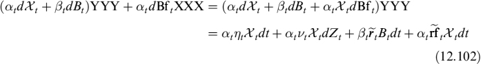
where ![]() and denomination in YYY has been omitted in the last line. Setting
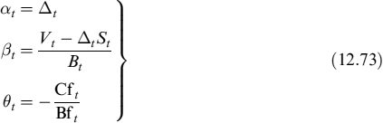
and denomination in YYY has been omitted in the last line. Setting ![]() and βt = (Vt − Ct − ΔtXt)/Bt, and following the same mathematical passages as in Section 12.1, we come up with the PDE:
and βt = (Vt − Ct − ΔtXt)/Bt, and following the same mathematical passages as in Section 12.1, we come up with the PDE:
From (12.103) we can easily derive the two ways of expressing the value of the contingent claim at time 0:
and
We have explicitly indicated the drift that the FX rate must have under the bank's replication measure. In equation (12.104) decomposition of the value of the collateralized contract is given as the sum of the otherwise identical non-collateralized deal and of LVA.
We introduce a further decomposition that can be used to allocate revenues and costs within a dealing room. We rewrite equation (12.103) as:

The solution to (12.106) is:
where VNC is the price of the non-collateralized contract assuming no funding spread, LVA is the liquidity value adjustment originated by the difference between the collateral and risk-free rates:
and, finally, FVA is the funding value adjustment due to the funding spread and paid to replicate the contract and the collateral account:
FVA can be decomposed according to the spread paid in YYY:
and the funding adjustment due to the spread paid in XXX:
Collateral posted in base currency
When collateral is posted in base currency XXX, we can apply the results derived above for a general derivative contract to an FX derivative contract. The replicating portfolio is built as follows
and its evolution is:
Choosing βt = (Vt − ΔtXt)/Bt and θ = − (Cft − Δt)/BftXXX = −(Ct − ΔtXt)/BftYYY, we derive the following PDE:
The solution is
Another solution to (12.114) is:
where VNC is the price of the non-collateralized contract assuming no funding spread, LVA is the liquidity value adjustment originated by the difference between the collateral and risk-free rates:
and, finally, FVA is the funding value adjustment due to the funding spread, which is paid to replicate the contract and the collateral account:
Value of an FX forward (outright) contract
Let us assume collateral is posted in YYY. A (long) FX forward contract, or outright, struck at level X has a terminal value:
so that applying the compact formula (12.105)
The value at inception of the contract is nil: if we disregard for the moment all the adjustments due to the default risk of the bank and its counterparty, we can price the contract and find level X = XC(t, T) that makes the value at the beginning of the contract zero with formula (12.104). If the bank needs to replicate a long position in the outright contract, then the outright price can easily be shown to be:
On the other hand, when the bank wants to replicate a short position, the outright price is:
Remark 12.2.2. In both cases, collateralization and, hence, the collateral rate do not affect the fair level of the outright contract, although LVA contributes to the value of the contract when the outright is seasoned and no longer at-the-money as at inception. On the contrary, funding spreads paid on either currency (YYY or XXX) enter into the formula and are crucial to defining both the replication value of the contract to the bank and the fair level.
Remark 12.2.3. Equation (12.106) makes it abundantly clear that we are still within a risk-neutral framework, where everything is discounted using the risk-free rate, and the drift of the FX rate process Xt is the difference between the numeraire and base currency: a standard result. Using PDE (12.103) leads to more convenient valuation formulae, but in our opinion makes it less clear how the value is composed or why it can be different to different parties, despite still working in a dynamic replication setting that produces a risk-neutral value.15
If collateral is posted in XXX, then the forward price is the level making the contract value at inception zero computed via PDE (12.114) whose solution can be written as the compact formula (12.115), so that
It is quite easy to check that both the long and short outright fair price level is the same as in formulae (12.121) and (12.122), so that XC(t, T) = XCf(t, T), with XCf the outright fair price at time t for maturity T when the collateral is posted in the base currency.
Remark 12.2.4. Although the fair level of the outright (FX forward) price is independent of the currency in which the collateral is posted, the value of the contract does depend on it. The values of two contracts one collateralised in the numeraire and the other in the base currency differ during their life, being equal (i.e., zero) only at inception and at expiry.
Replication with FX swap
The funding spread in both currencies can be strongly abated if the bank uses collateralized instead of unsecured lending. In the FX this can easily be achieved via an FX swap, which is in all respects equal to a repo traded in other markets. The FX swap is the sum of a spot contract plus an outright, but it can also be seen as the borrowing/lending of an XXX amount against collateral represented by the YYY amount.16
FX swaps for given expiry T are quoted in the market in points over the spot rate X, so that the level at which the outright is traded is defined as F(t, T) = X′ + p(t, T), where p(t, T) are the swap points prevailing at time t for an FX swap expiring at time T.17 The outright level also defines the FX swap implied rate, which mainly depends on the differential between the numeraire and the base currency, but there are other factors (even beyond credit risk) that determine the generally defined cross-currency basis. The implied FX swap (continuous) rate is defined as:
Using an FX swap to replicate the FX derivative contract and assuming for the moment that it is CSA-collateralized in YYY, formula (12.102) is modified as follows:
Setting ![]() and βt = (Vt − Ct), the evaluation PDE becomes:
and βt = (Vt − Ct), the evaluation PDE becomes:
The solution to (12.126) is:
where, again, VNC is the price of the non-collateralized contract on exchange rate X, assuming no funding spread and repo rate; LVA is the liquidity value adjustment due to the collateral agreement:
![]()
and FVA is the funding value adjustment:
where FVA is split into two parts: the funding cost needed to finance collateral ![]() and the spread of the repo rate over the risk-free rate
and the spread of the repo rate over the risk-free rate ![]() paid on the position of amount Δt of the underlying asset.
paid on the position of amount Δt of the underlying asset.
It is possible to rewrite (12.127) in a more convenient fashion for computational purposes:
The FX swap can be used to replicate the outright contract shown above: in the end the FX swap is just the replication strategy of an outright operated with a single counterparty, thus minimizing loss given defaults and hence the spread paid. Keeping in mind that the FX swap, being a derivative contract itself, is CSA-collateralized, we also get the same cash flow profile for both the outright and the FX swap, so that funding spreads should not be considered in the evaluation process. The replica of the contract is then independent of the creditworthiness of the replicator bank. This means that, in practice, they are the same contract when a CSA agreement is in operation and that the outright fair price is just the FX swap price:
The dynamics for the FX rate, when replication is operated via the FX swap, are:
Let us now see what happens if replication is performed using a repo contract and the collateral is posted in the base currency (XXX). Equation (12.113) modifies as follows:
Setting βt = Vt/Bt and θ = −Cft/BftXXX = − Ct/BftYYY, we derive the following PDE:
where ![]() . The solution to (12.133) is:
. The solution to (12.133) is:
where, as usual, VNC is the price of the non-collateralized contract on the exchange rate X, assuming no funding spread and repo rate, LVA is the liquidity value adjustment due to the collateral agreement:
![]()
and FVA is the funding value adjustment:
with ![]() as above. A compact solution in this case is:
as above. A compact solution in this case is:
It is clear that the currency of the collateral is immaterial when a FX swap is used to replicate a forward contract, since from (12.136) we can derive the fair outright level when collateral is posted in the base currency, which is the same as in (12.130), so that: XCf = XC.
12.2.3 Interest rate derivatives
We argued above that interest rate derivatives should be considered as primary securities, so that pricing formula cannot be derived by a true replication argument, but they are simply market pricing formulae. We illustrate how to evaluate two basic contracts of the interest rate derivative market: a forward rate agreement (FRA) and an interest rate swap (IRS).
Forward rate agreement
Assume we have the risk-free discount curve in both currencies denoted by D and Df, respectively, for YYY and XXX. The pricing formula for a FRA written on Libor rate Li(Ti−1) in YYY, but with collateral posted in XXX can be written in much the same way as that presented above for contracts on other underlying assets and derived from a replication argument:
that is, the expected Libor rate under the Ti forward measure of the value of the contract at expiry Ti−1 plus the LVA. We used Ti = Ti − Ti−1 in equation (12.137).
LVA is the present value of the difference between the risk-free rate ![]() and the collateral rate
and the collateral rate ![]() , fixed at date tj−1 and valid until date tj, both for currency XXX, applied to fraction γ of the value of contract FRA(tj; Ti−1, T2) for a total of N days between t and the forward settlement T1, so that tN = T1:
, fixed at date tj−1 and valid until date tj, both for currency XXX, applied to fraction γ of the value of contract FRA(tj; Ti−1, T2) for a total of N days between t and the forward settlement T1, so that tN = T1:

where ![]() is the difference in the fraction into which the year is split between two rebalancing times of the collateral (typically, one day). Let us assume that market quotes for FRAs refer to when LVA is nil, implying that the collateral rate is supposed to be risk-free rate LDf(t; tj−1, tj) = Of (t; tj−1, tj) for all j: this is not unreasonable given that the standard CSA between banks provides for remuneration of the collateral account at the OIS rate and the latter can be considered a very good proxy for the risk-free rate. Equation (12.137) will then be:
is the difference in the fraction into which the year is split between two rebalancing times of the collateral (typically, one day). Let us assume that market quotes for FRAs refer to when LVA is nil, implying that the collateral rate is supposed to be risk-free rate LDf(t; tj−1, tj) = Of (t; tj−1, tj) for all j: this is not unreasonable given that the standard CSA between banks provides for remuneration of the collateral account at the OIS rate and the latter can be considered a very good proxy for the risk-free rate. Equation (12.137) will then be:
which is exactly the same result as given in Section 12.1 and of the current pricing theory based on a multi-curve setup.18 The FRA fair rate is the expected value of Libor at the settlement date of the contract, under the expiry Ti forward risk measure:
According to market conventions, the contract actually settles the present value of payoff Ti at Ti−1 using the FRA fair rate in (12.140), since the latter is corrected by a convexity adjustment as discussed in [91]. The adjustment is nevertheless quite small (a fraction of a basis point).
Let us now assume the collateral agreement provides for remuneration of collateral different from the OIS rate: setting ![]() equal to the spread between the daily risk-free rate and collateral rate in XXX, and assuming it is a stochastic process independent of the value of the FRA, we can rewrite equation (12.138) as:
equal to the spread between the daily risk-free rate and collateral rate in XXX, and assuming it is a stochastic process independent of the value of the FRA, we can rewrite equation (12.138) as:

The second expectation in (12.141) is ![]() , so that we finally get:
, so that we finally get:

Apart from a slight change of notation, the results are the same as in [45] and this is also the case when we consider FVA. To this end, define ![]() as the funding rate paid by the bank in XXX. When financing the collateral (i.e., when the NPV of the contract is negative) the bank has to pay this rate and receive the collateral rate, whereas in the opposite situation (i.e., positive NPV), then it invests the collateral received at the risk-free rate, paying the collateral rate. Let the funding spread over the risk-free rate be
as the funding rate paid by the bank in XXX. When financing the collateral (i.e., when the NPV of the contract is negative) the bank has to pay this rate and receive the collateral rate, whereas in the opposite situation (i.e., positive NPV), then it invests the collateral received at the risk-free rate, paying the collateral rate. Let the funding spread over the risk-free rate be ![]() : we further assume that it is not correlated with the NPV of the FRA. FVA is:
: we further assume that it is not correlated with the NPV of the FRA. FVA is:
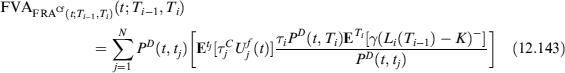
where E[X−] = E[min(X, 0)]. It is straightforward to show that:

where Floorlet(tj; Ti−1, Ti, K) is the price of a floorlet priced at time tj, expiry at Ti−1, settlement at Ti, with strike K. If the bank has a short position in the FRA, then FVA is

where Caplet(ti; Ti−1, Ti, K) is the price of a caplet and the arguments of the function are the same as for the floorlet. The total value of the FRA is:

The fair rate making the value of the contract at inception zero has to be computed recursively.
Remark 12.2.5. Formula (12.139) shows that the FRA fair rate is independent of the currency in which the collateral is posted: this is the same as the result derived above for derivatives with different underlying assets that can be replicated by a dynamic strategy. The difference between FRA fair rates relating to contracts collateralized in two different currencies can be caused by more difficult access to the money market in XXX for banks operating in the domestic country (where YYY is the currency used). This will produce generalized and higher funding costs borne by domestic banks when posting collateral in the foreign currency, so that an average FVA, typically paid by all banks, is added to the XXX-collateralized FRA. In this case the FRA fair rate will be dependent on the currency chosen to post the collateral.
Interest rate swap
We will not devote much space to the results for an IRS since they are derived in much the same way as those for a FRA and are in any event the same as in Section 12.1 (to which we refer the reader for more details).
Consider an IRS whose fixed leg pays rate K on dates ![]() ; the floating leg receives Libor fixings on dates Ta, …, Tb. We assume that the set of floating rate dates includes the set of fixed rate dates. For both legs the present value of these payments is obtained by discounting them using the YYY discount curve D. If collateral is posted in XXX, the value at time t of the IRS is:
; the floating leg receives Libor fixings on dates Ta, …, Tb. We assume that the set of floating rate dates includes the set of fixed rate dates. For both legs the present value of these payments is obtained by discounting them using the YYY discount curve D. If collateral is posted in XXX, the value at time t of the IRS is:
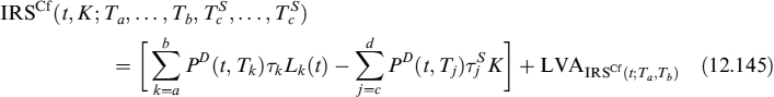
with:

where ![]() . LVA is as usual the difference between the XXX currency's risk-free rate and the collateral rate applied to fraction γ of the NPV, for a total of N days occurring between valuation date t and the end of the contract tN = Tb. As far as swaps are concerned, we can also make the assumption that market quotes refer to the situation when LVA = 0, implying that the XXX currency's risk-free and collateral rates are the same. When the two rates are different, LVA is:
. LVA is as usual the difference between the XXX currency's risk-free rate and the collateral rate applied to fraction γ of the NPV, for a total of N days occurring between valuation date t and the end of the contract tN = Tb. As far as swaps are concerned, we can also make the assumption that market quotes refer to the situation when LVA = 0, implying that the XXX currency's risk-free and collateral rates are the same. When the two rates are different, LVA is:

The second expectation in (12.141) is ![]() , where Ea,b is the expectation taken under the swap measure, with the numeraire equal to annuity
, where Ea,b is the expectation taken under the swap measure, with the numeraire equal to annuity ![]() . So, we can write:
. So, we can write:

FVA is defined analogously to the FRA case:

Introducing options on swaps, the second expectation in (12.149) is:
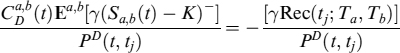
where Rec(t; Ta, Tb) is the price of a receiver swaption priced at time tj, expiry at Ta, on a swap starting at Ta and maturing at Tb, with strike K. If the bank has a short position in the IRS (i.e., it is a fixed rate receiver), then FVA is
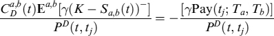
where Pay(t; Ta, Tb) is the price of a payer swaption. So, the total value of the IRS can be written as:
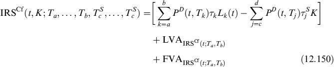
It is worthy of note that fair market swap rates are also independent of the currency used to post collateral, although the same considerations as those in Remark 12.2.5 apply.
12.2.4 Cross-currency swaps
Cross-currency swaps (CCS) involve at least two currencies since they are the periodic exchange of Libor rates in one currency against the Libor rates of another currency, usually with a basis spread paid over one of them. Most CCS are against US dollars, and the basis spread quoted in the market is paid over the Libor of the other currency of the deal. We now learn how to price a CCS when collateral is posted in US dollars, which we name “major currency” in what follows and which can be thought of as XXX introduced above.19 The other currency is named “minor currency” and is YYY as before. To avoid any confusion, we will add superscript X or Y to refer to the relative currency whenever needed.
Let Tb be the expiry of a swap starting at Ta with fixed rate Sa,b(t). Let ![]() be the forward Libor rate corresponding to the payment frequency of the floating leg (e.g., 6-month Libor for semiannual payments) for the period between Tk−1 and Tk, computed at time t, with Tk ≥ Ta and Ta ≤ t < Tk. The notation is the same as above. PDx (t, v) is the US risk-free discount factor for the period t to v. If
be the forward Libor rate corresponding to the payment frequency of the floating leg (e.g., 6-month Libor for semiannual payments) for the period between Tk−1 and Tk, computed at time t, with Tk ≥ Ta and Ta ≤ t < Tk. The notation is the same as above. PDx (t, v) is the US risk-free discount factor for the period t to v. If ![]() is the fair market rate of the swap, the IRS can be computed under the assumption of nil LVA, so that:
is the fair market rate of the swap, the IRS can be computed under the assumption of nil LVA, so that:
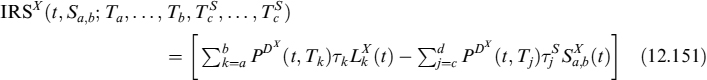
The swap is collateralized in XXX. The first term in the sum on the right-hand side is the present value of the stream of floating rate cash flows, whereas the second is the present value of fixed leg payments. The sum is nil for par swaps. We indicate the present value of the floating leg by ![]() , such indication will be found convenient in what follows. We can define in much the same way an IRS in minor currency, collateralized in major currency, with fair swap rate
, such indication will be found convenient in what follows. We can define in much the same way an IRS in minor currency, collateralized in major currency, with fair swap rate ![]() .
.
Let ![]() be a cross-currency swap against the US dollar, with the same start Ta, maturity Tb and frequency as the standard IRS in (12.151) for both floating legs denominated in the two currencies;
be a cross-currency swap against the US dollar, with the same start Ta, maturity Tb and frequency as the standard IRS in (12.151) for both floating legs denominated in the two currencies; ![]() is the basis paid over Libor LY of the minor currency leg. Collateral is posted in US dollars (or XXX). The value of the YYY-receiver CCS, keeping LVA and FVA in mind, is:
is the basis paid over Libor LY of the minor currency leg. Collateral is posted in US dollars (or XXX). The value of the YYY-receiver CCS, keeping LVA and FVA in mind, is:
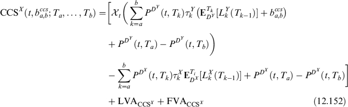
Let us focus on the first three lines of (12.152) (i.e., the part in square brackets) and postpone for the moment our analysis of the LVACCS. To price a CCS, it is convenient to adopt the vantage point of an agent operating in the major (USD) currency economy. Therefore, we need to know how to evaluate a Libor payment in the minor currency when seen from the major-currency economy.
To this end, assume we have at time t = 0 (i) discount factors PDX (0, T) for the major currency, (ii) a minor-currency par swap rate paying ![]() with the swap collateralized in the major currency and cross-currency basis swap spreads
with the swap collateralized in the major currency and cross-currency basis swap spreads ![]() and (iii) the spot exchange rate X (i.e., the number of minor-currency units equal to 1 unit of the major currency). For simplicity we consider the same schedule for all legs. We can establish the following relationship.
and (iii) the spot exchange rate X (i.e., the number of minor-currency units equal to 1 unit of the major currency). For simplicity we consider the same schedule for all legs. We can establish the following relationship.
Proposition 12.2.1. When collateral is in a major currency, the following equation holds:
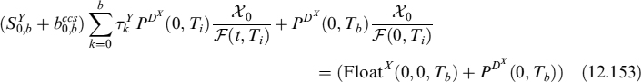
Proof. Let us consider the following portfolio, which contains a set of transactions and its associated cash flows, disregarding the effects of collateral, for a swap starting at time t = 0, and with all T = 1 to lighten the notation:
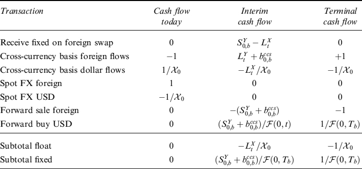
Since collateral from all contracts is posted in the major currency, the collateral of net cash flows is by assumption posted in the major currency as well. These net cash flows resemble those of a swap of major-currency Libor against a schedule of fixed payments. Therefore, from the results derived above for an IRS, net stated cash flows can be valued by discounting them at the major-currency risk-free rate.
The present value of paying Libor on notional 1/X0 and a terminal payment of 1/X0 is obviously ![]() . Since there are no net cash flows at time t = 0, total present value of the two subtotal cash flows must equal 0. Therefore:
. Since there are no net cash flows at time t = 0, total present value of the two subtotal cash flows must equal 0. Therefore:
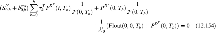
Multiplying all terms by X0, to express everything in minor-currency units, and rearranging yields the desired result.
Remark 12.2.6. From the analysis conducted above for standard IRSs collateralized in some other currency, the fair swap rate ![]() can be considered as independent of the choice of collateral currency, since LVA is unaffected. We already stressed in Remark 12.2.5 that it may be possible for the fair FRA and IRS rates to differ according to the choice of currency used to post collateral. So, if different IRSs are quoted in the market for the different possible currencies in which the collateral is posted, we can use these quotes for
can be considered as independent of the choice of collateral currency, since LVA is unaffected. We already stressed in Remark 12.2.5 that it may be possible for the fair FRA and IRS rates to differ according to the choice of currency used to post collateral. So, if different IRSs are quoted in the market for the different possible currencies in which the collateral is posted, we can use these quotes for ![]() in equation (12.153). Otherwise, we can quite safely assume that swap rates for IRSs collateralized in a minor currency are the same for any other collateral currency.
in equation (12.153). Otherwise, we can quite safely assume that swap rates for IRSs collateralized in a minor currency are the same for any other collateral currency.
It is straightforward to derive the present value of receiving Libor rates in a minor currency from a major-currency perspective: since foreign par swaps are fair the value of fixed cash flows must equal the value of floating cash flows. The value of fixed cash flows, from (12.153), is ![]() , so that:
, so that:
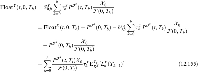
So, we are able to switch to a major-currency Tk forward measure for each minor-currency Libor rate. This allows us to price a CCS collateralized in the major currency, since we can insert equation (12.155) into (12.152), setting t = Ta = 0:
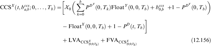
LVA is defined as:

where the notation is the same as above. FVA is defined similarly as:

Remark 12.2.7. The setup outlined above allows consistent valuation of IRSs in different currencies and of CCSs. from (12.153) we can derive the term structure of implied FX swap levels. These are then used in (12.155) to bootstrap YYY Libors seen from the XXX economy perspective: they guarantee that CCSs are repriced correctly. So, in this approach we do not build a basis-adjusted discount curve to match CCS prices, a method usually adopted in practice in many banks. We prefer to build, in our opinion more consistently, adjusted Libor projection curves and leave discount curves unchanged. By definition, IRSs in the two currencies are correctly repriced as long as proper discount and projection curves are used.
12.3 VALUATION OF NON-COLLATERALIZED INTEREST RATE SWAPS INCLUDING FUNDING COSTS
In Chapter 10 we correctly defined the debit value adjustment (DVA) of a derivative contract and put forward a definition that declares the DVA worsens contract conditions for a counterparty because it has to compensate the other party for the possibility of its own default. DVA is very strictly linked to funding costs (FCs) when the contract is a loan, a bond or more generally some kind of borrowing. The link is much less tight (maybe even nonexistent) for some derivative contracts such as swaps. The funding costs for a derivative contract is actually the DVA (plus liquidity premium and intermediation cost, if priced in market quotes) that a counterparty has to pay on the loan contracts it has to close to fund, if needed, negative cumulated cash flows until maturity.
In what follows we study how to include funding costs in the valuation of interest rate swaps (IRSs) and show how they affect the value of the swap via funding value adjustment (FVA), in analogy to credit value adjustment (CVA) and DVA. We consider valuation of IRS contracts in the absence of collateral agreement or any other form of credit risk mitigation.
IRS valuation effectively demonstrates how the inclusion of funding costs makes even relatively simple contracts very complex especially when all the relevant risks are considered.
12.3.1 The basic setup
Let us assume that, at time t, we want to price a very general (nonstandard) swap, such as an amortizing or zero-coupon swap, with possibly different amounts for the fixed and floating rates, and accompanied, possibly, by a time-varying fixed rate.
Let us introduce the meta-swap, which is a swap with unit notional and a time-varying fixed rate that is equivalent to the contract fixed rate times the notional amount for each date ![]() (i.e., the one at the start of the calculation period). The start date of the swap is Ta and the end date is Tb.
(i.e., the one at the start of the calculation period). The start date of the swap is Ta and the end date is Tb.
Let us assume that the swap's floating leg pays at times Ta+1, …, Tb, where Ta+1 is the first fixing time (dates are equally spaced acording to floating leg payment frequency); Fi(t) are the forward rates, as at time t, paid at time Ti and fixed at Ti−1, for a + 1 ≤ i ≤ b; the swap's fixed leg pays at times Tc1, …, TcJ, where c1 ≥ a and cJ = b. Fixed leg times are assumed to be included in the set of floating leg times and this is usually the case for standard swaps quoted in the OTC market, for which floating flows are paid semiannually or quarterly, whereas fixed flows are paid annually.
The fixed rate payment at each payment date Tcj is:
where
and ![]() denotes the fraction into which the year is divided (or year fraction) between payment dates for the fixed leg.
denotes the fraction into which the year is divided (or year fraction) between payment dates for the fixed leg.
The floating leg will exchange future Libor fixing times αi, which is the year fraction times the notional ![]() at the beginning of the calculation period:
at the beginning of the calculation period:
Note that despite the fact that the meta-swap has unit notional, both the total fixed rate and the year fraction contain the notional of the swap.
Define
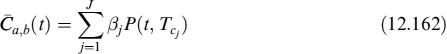
as the annuity, or DV01 in market lore, of the meta-swap. We assume ![]() . Discount factors (or discount bonds) P(t, T) are taken from a risk-free curve; in the current market environment, the best approximation to the risk-free rate is given by overnight rates. An entire curve based on these rates can be bootstrapped from OIS swaps. Define also:
. Discount factors (or discount bonds) P(t, T) are taken from a risk-free curve; in the current market environment, the best approximation to the risk-free rate is given by overnight rates. An entire curve based on these rates can be bootstrapped from OIS swaps. Define also:
We then have:
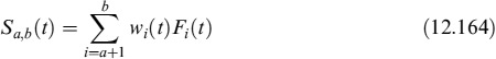
which is the swap rate Swpa,b(t) = 0 that makes the value of the meta-swap at t equal zero (Swpa,b(t) is the value at time t of a swap starting at Ta and terminating at Tb). In a standard swap the fair rate is the average forward Libor rate Fi weighted as a function of discount factors. In the case of the meta-swap the average forward Libor rate is weighted as a function of the notionals and discount factors. It is easily checked that this is the rate making the present value of the floating leg equal to that of the fixed leg. Note that the risk-free rates used to derive discount factors are not the same as those used to determine Libor forward rates Fi.20
Some points are worth stressing here. First, pricing is correct if both counterparties involved are risk free; second, since at least one of the two counterparties is usually a bank, the fact that Libor rates are above risk-free rates is in conflict with the first point, Libor being rates applied to unsecured lending to an ideal bank with a good credit rating, but not risk free in any case; third, as a consequence of the second point, full risk pricing should also include credit adjustments (CVA and DVA) as compensation for default risk relating to either party.
To isolate the funding component of the value of a swap, we consider an abstraction and disregard adjustments due to counterparty credit risk. We will include counterparty credit risk later on. To help us analyse the problem linked to the cost of funding, we first introduce a hedging strategy for the swap and then analyse the cash flows implied by it.
12.3.2 Hedging swap exposures and cash flows
Assume a bank takes a position in a swap starting at Ta and ending at Tb that can be described by the general formulae given above: the fair swap rate is ![]() . The swap can either be a fixed rate payer or fixed rate receiver, in which case the fixed leg has a negative (positive) sign. The bank wants to hedge exposures to interest rates, but at the same time wants to come up with a well-defined, possibly deterministic schedule of cash flows so as to plan its funding and/or investment. To lock in future cash flows, we suggest the following strategy:
. The swap can either be a fixed rate payer or fixed rate receiver, in which case the fixed leg has a negative (positive) sign. The bank wants to hedge exposures to interest rates, but at the same time wants to come up with a well-defined, possibly deterministic schedule of cash flows so as to plan its funding and/or investment. To lock in future cash flows, we suggest the following strategy:
- take stock of all dates Tc1, …, TcJ when fixed leg payments occur;
- close (forward) starting swaps Swp (Tci−1, Tci.), for i = 1, …, J using fixed rate payments opposite to those of the swap the bank wants to hedge (the fair rate for each swap is
 ).
).
Let cf (Tk) be the amount of cash to receive or pay at time Tk, generated by the hedged portfolio above. The floating leg of each hedging swap balances the floating leg of the meta-swap for the corresponding period so that at each time Ti, with a + 1 ≤ i ≤ b we have cf (Ti) = 0. On the dates Tcj, for 1 ≤ j ≤ J, when the fixed legs of the total portfolio (comprising the meta-swap and hedging swaps) are paid, the net cash flows are:
![]()
where 1{R} (respectively, 1{P}) is the indicator function equal to 1 if the swap is receiver (respectively, payer).
Furthermore, let CF(Ta, Tcj) be the compounded cumulated cash flows from the start time Ta up to time Tcj via the recurrent equation:
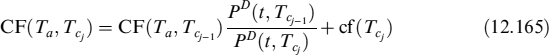
with the starting value CF(Ta, Ta) = 0.
Cash flows are assumed to be reinvested at the risk-free rate: this is possible if the cumulated cash flows start at zero, increase and do not become negative. We indicate by cf±(ck) a positive/negative cash flow, whereas we indicate by ![]() the maximum number of cumulated cash flows between start date Ta and end date Tb:
the maximum number of cumulated cash flows between start date Ta and end date Tb:
Analogously, we denote by CF(Ta, Tb) the minimum number of cumulated cash flows:
For standard market swaps, we generally have two possible patterns of cumulated cash flows, depending on the side of the swap (fixed rate payer/receiver) and on the shape of the term structure of interest rates: the first pattern is always negative, while the second is always positive. This means that ![]() is zero and CF(Ta, Tb) is a negative number in the first case; in the second case CF(a, b) is zero and
is zero and CF(Ta, Tb) is a negative number in the first case; in the second case CF(a, b) is zero and ![]() is a positive number. For funding costs to be included in the pricing, we need only focus on the first case, whereas the second case poses no problems. In fact, in the second case, the cash flows generated internally within the deal, including their reinvestment in a risk-free asset, imply no need to resort to additional funding. This is not true in the first case.
is a positive number. For funding costs to be included in the pricing, we need only focus on the first case, whereas the second case poses no problems. In fact, in the second case, the cash flows generated internally within the deal, including their reinvestment in a risk-free asset, imply no need to resort to additional funding. This is not true in the first case.
Negative cash flows need to be funded and related costs should be included in the pricing. As mentioned above, we disregard the effect of the defaults of either parties on funding costs for the moment: we will consider this later.
Now, given the market term structure of forward Libor rates, a swap usually implies for a counterparty a string of negative cash flows compensated by a subsequent string of positive cash flows. The present (or, equivalently, the future at expiry) value of negative cash flows is equal to the present (or future) value of positive cash flows, provided there is no default by either counterparty and that each counterparty is able to lend and borrow money at the risk-free rate.
If we assume that it is possible for the counterparties to lend money at the risk-free rate, but that they have to pay a funding spread over the risk-free rate to borrow money, then the problem of how to correctly consider this cost arises. We suggest two strategies to fund negative cash flows, the second one has two variants. We examine them separately from the perspective of one of the two parties (say, the bank), whereas the other party is assumed to be a client that is unable to transfer his funding costs to the pricing.
12.3.3 Funding spread modelling
To keep things simple, let us assume that the funding spread is due only to credit factors and that there are no liquidity premiums. More specifically, the bank has to pay a spread that originates from its default probability and loss given default. If we assume that after default a fraction R of the market value of the contract is immediately paid to the counterparty – recovery of market value (RMV) assumption – then we have a very convenient definition of the instantaneous spread21 as st = (1 − R) λt, where λ is default intensity (i.e., the jump intensity of a Poisson process, default being the first jump). We choose a doubly stochastic intensity model so that the survival probability between time 0 and time T is given by (see Chapter 8):
![]()
where default intensity λt is a stochastic process that is assumed to be defined by CIR-type dynamics as in equation (8.140). In this setting, SP(0, T) has the closed-form solution given in equation (8.141).
The formula to compute spread discount factors is readily shown to be the same as for survival probability with a slight change in parameters:
where we used properties inherent in the CIR process.22
Let PD(0, T) be the price at 0 of a default risk-free zero-coupon bond (bootstrapped from the OIS swap curve, for example) maturing at T; the price of a correspondent zero-coupon bond issued by the bank is PB(0, T) = PD(0, T)Ps(0, T) (where we have omitted some parameters of function Ps(0, T) to lighten the notation), assuming default intensity as given by the dynamics in (8.140) and a recovery rate R. This is also the discount factor used to compute the present value of money borrowed by the bank and should be considered effective at embedding funding costs.23
12.3.4 Strategy 1: Funding all cash flows at inception
The first strategy is based on the idea of funding all negative cash flows from the very inception of the swap. To this end, we compute the minimum cumulated amount CF(a, b) over the entire duration of the swap [Ta, Tb]. Assuming that CF(a, b) < 0, this implies a certain amount of cash that needs to be entirely funded at inception. The idea is to borrow money and then use the cash flows generated by the hedged swap portfolio to repay it, possibly according to a predefined amortization schedule determined by the cash flow pattern. We need to consider some relevant practical matters too:
- The total sum entirely funded at inception can be invested in a risk-free asset (a zero-coupon bond issued by a risk-free counterparty,24 for example). The amounts needed when negative cash flows occur can be obtained by selling back a fraction of the investment. The interest earned has to be included in the pricing.
- The funding for long maturities can be done with a loan that the bank trades with another counterparty; this usually implies periodic payment of interest on the outstanding amount. Periodic paid interest also needs to be included in the evaluation process.
To formalize all this, let us consider the bank pays annual interest on the outstanding of the borrowed amount on an annual basis, according to a fixed rate calculated at the start keeping the probability of default in mind. We assume that the bank pays a fraction of the market value of the loan should it default.
Let t = 0 and A be the initial amount of a loan that expires at Tb (equal to expiry of the swap) and has a capital and interest payment schedule at dates [Td1, …, TdM]: we assume that this set also contains the set of payment dates for the fixed leg of the swaps. We define capital payment of loan A at time Tk as K(Tdk) = A(Tdk) − A(Tdk−1), with A(t) = A, A(Tb) = 0 and ![]() . Note that the loan starts at the inception of contract t, which could even be before the start of swap Ta; moreover, interest payments can also occur before Ta. Let
. Note that the loan starts at the inception of contract t, which could even be before the start of swap Ta; moreover, interest payments can also occur before Ta. Let ![]() be the fixed rate that the bank has to pay on this loan: it can be derived from the following relationship
be the fixed rate that the bank has to pay on this loan: it can be derived from the following relationship
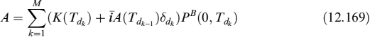
where δdk = Tk − Tk−1 is the accrual period. Discounting is carried out by means of discount factors PB(T0, Tk) such that the losses the lender suffers on the bank's default can also be taken into account. From the bank's perspective the spread paid over the risk-free rate is a funding cost, whereas it is compensation for the default risk borne from the lender's perspective.25 The loan's fair fixed rate ![]() is:
is:
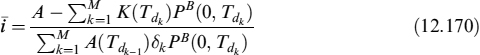
As mentioned above, once the amount of loan A is received by the bank at time 0, it can be reinvested at the risk-free rate and partially reduced to cover future outflows of cash when they occur. Let us define available liquidity at time Tdk via the recurrent equation:

with AVL(0) = A. Equation (12.171) states that liquidity available to the bank at time Tdk is liquidity available at the previous time Tdk−1 invested at the forward risk-free rate over the period [Tdk−1, Tdk], plus the cash flow occurring at time Tdk, minus the sum of instalment and interest rate payments. Cash flows can either be positive or negative. When positive cash flow cf(Tdk) > 0 occurs, it is used to abate the outstanding amount of the loan; on the other hand, when negative cash flow cf (Tdk) < 0 occurs, then there is no capital instalment and K(Tdk) = 0. Since it is possible to lock in future cash flows at contract inception via the suggested hedging portfolio, the amortization plan for the loan, however irregular it may be, can be established at time t = 0. The amortization plan can then be defined as:
A(Tdk) = A(Tdk−1) − cf+(Tdk)
The amount of the loan the bank has to borrow will be a function of the term structure of Libor interest rates and of bank funding spreads, the fixed leg notional schedule of the swap and the fixed rate of the swap:
![]()
where sk(t) is the funding spread for period [Tk−1, Tk]. Amount A has to be determined so as to satisfy two constraints:
- Available liquidity AVL(Tdk) at each time Tdk must always be positive, so that no other funding is required until the end of the swap. This constraint is satisfied if
 (i.e., if it is at least equal to the sum of negative cash flows occurring in the future).
 - At the maturity of swap Tb available liquidity should be entirely used to finance all negative cash flows, so that AVL(Tb) = 0, thus minimizing funding costs (assuming no unnecessary funding at inception has been requested by the bank).
Amount A can be determined very quickly numerically. Given a positive funding spread, the positive cash flows originated by the hedged portfolio will not be sufficient to cover the loan's amortization plan, so that on the last capital instalment date extra cash must be provided by the bank to pay back its debt in its entirety; ultimately, this represents a cost that has to be included in the pricing of the swap. Let FC be the present value of this cost. It can then be added to the fair swap rate as follows:
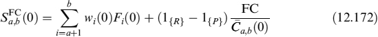
where annuity ![]() and weights wi(0) are defined as in (12.162) and (12.163). Equation (12.172) increases (decreases) the fair swap rate if the bank is a fixed rate receiver (payer) in the contract, thus compensating the extra costs due to funding costs.
and weights wi(0) are defined as in (12.162) and (12.163). Equation (12.172) increases (decreases) the fair swap rate if the bank is a fixed rate receiver (payer) in the contract, thus compensating the extra costs due to funding costs.
Since the amount of loan A is a function of swap rate Sa,b(0), which in turn is affected by funding cost FC that depends of A, a numerical search is needed to determine the final fair swap rate ![]() , which makes both the available liquidity and the FC equal to zero. Convergence is typically achieved in a few steps.
, which makes both the available liquidity and the FC equal to zero. Convergence is typically achieved in a few steps.
The value of the swap, when the rate is ![]() , is:
, is:
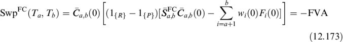
since for payer (receiver) swap ![]() , the swap has a positive value that equates the reverse sign FVA, which is the quantity that makes the swap value nil at inception when funding costs are included in the pricing.
, the swap has a positive value that equates the reverse sign FVA, which is the quantity that makes the swap value nil at inception when funding costs are included in the pricing.
12.3.5 Strategy 2: Funding negative cash flows when they occur
The second strategy we propose involves matching negative cash flows when they occur by resorting to new debt, given that cumulated cash flows are not positive and/or insufficient. The debt is carried on by rolling it over and paying a periodic interest rate plus a funding spread; moreover, it can be increased when new negative cash flows occur and decreased when positive cash flows are received. Interest rates and funding spreads paid are those prevailing in the market at the time of rollover, so that they are not fixed at inception of the contract.
The advantage this strategy has over the first is that the bank borrows money only when necessary and does not have to pay any interest and funding spread for the time preceding cumulated cash flows becoming negative. On the other hand, the bank is exposed to liquidity shortage risks and to uncertain funding costs that cannot be locked in at the start of the contract. The latter statement will become clearer in what follows.
Let us assume that the hedged swap portfolio generates at given time Tk a negative cash flow cf− (Tk) and that cumulated cash flows are negative: the bank funds the outflow by borrowing money in the interbank market. We assume that the debt is rolled over in the future and that the bank pays interest plus a funding spread over period [Tk, Tk+1]; the borrowed amount varies depending on the cash flow available at time Tk+1. Hence, the debt evolves according to the following recurrent equation:

Note we are using defaultable discount factors to include interest payments over period [Tdk, Tdk+1]. This means we are forecasting the future total interest paid by the bank as forward rates implicit in the Libor rates and funding spreads at time t = 0. If the credit spread of the bank is positive, the positive cash flows generated by the hedged portfolio will not be enough to cover payback of the debt and related funding costs in their entirety. The terminal amount left is, as in the first strategy, a cost that the bank has to pay as it is strictly related to its credit spread. Ultimately, this is a funding cost to include in the pricing of the swap.
The Libor component of the total interest rate paid can be hedged by market instruments (e.g., OIS swaps) such that implicit forward rates can be locked in. There is another component, though, that has to be considered: the forward funding spread implicit in defaultable bond prices cannot be locked in easily at the start of the swap contract: this would entail the bank trading credit derivatives on its own debt, which is either impossible (in the case of CDSs) or difficult (in the case of spread options). The unexpected funding cost, due to volatility of the credit spread of the bank, has to be measured in any event and should also be included in the pricing. We suggest two possible approaches to measure unexpected future funding costs.
Measuring unexpected funding costs via spread options
The first approach is the measurement of unexpected funding costs via spread options. Let us assume rollover of debt is operated at dates [Td1, …, TdM], a set that also contains the set of payment dates of the fixed leg of the swaps. The forward rate, computed at t, paid on the outstanding debt at given date Tdk is:
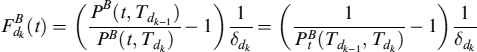
where ![]() is the forward price of a defaultable bond calculated at t. Expected debt rollover at time Tdk is:
is the forward price of a defaultable bond calculated at t. Expected debt rollover at time Tdk is:
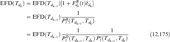
with EFD(Tdk−1) = FDB(Tdk−1).
Let sdk(t) be the forward funding spread, linked to the spread discount factor as follows:
so that
As pointed out above, this is simply expected rollover running parallel with expected funding spread (under the forward risk survival measure26). The rollover of debt carried out by compounding it at an unexpected funding spread level has to be considered; it can be written as:
Equation (12.178) expresses the unexpected funding cost to apply to roll over outstanding debt as a call spread option, with strike equal to the forward spread calculated at time t. Clearly, we are interested in cases when the spread is above the expected forward level: if it is actually lower, then the bank will pay less than expected, but we do not consider this potential benefit here. It is possible, with a little algebra, to rewrite the equation in terms of an option on a discount bond:
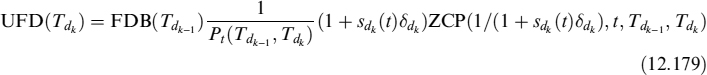
where ZCP is the future value computed at t of a put option with expiry Tdk−1 on a zero-coupon bond maturing at Tdk, struck at 1/(1 + sdk(t)δdk). The option is computed under the assumption that default intensity is a mean-reverting square root process, as described above. The solution for the present value of a put option expiring at T, written on a bond expiring at S, is provided in equation (8.40). If recovery rate R is different from 0, then the formula's parameters have to be adjusted as follows:
![]()
The future value of the put option on the spread's zero-coupon bond is:
![]()
which inserted in (12.179) yields:
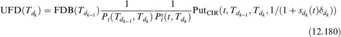
Total funding cost is the present value of the amount of the debt left at expiry of the swap (according to expected rollover) that has to be covered by the bank and hence is a cost, plus the present value of the spread options needed to hedge unexpected funding costs for each period:

This quantity is then used to determine the fair swap rate, via a numerical search as in equation (12.172): this is the rate making the present value of the funding cost FC = 0.
Measuring unexpected funding costs with a confidence level
The second approach to measuring unexpected funding costs is justified by the bank's difficulty to buy options on its own credit spread. This is the reason we suggest considering unexpected cost as a loss that cannot be hedged and that has to be covered by economic capital, similarly to VaR methodology.
Expected funding cost is still the same as in formula (12.175). Unexpected cost is computed by

The price of the spread discount bond Ps* (t, Tdk−1) is computed at a given confidence level (say, 99%). Since the probability of default follows a square root mean-reverting process at time t, the distribution at future time t′ of different levels of default intensity λt is known to be a non-central χ2 distribution.27 This allows us to compute, at a given date, the maximum level (with a predefined confidence level) of default intensity λt and hence the maximum level of the spread and total cost of refunding each funding source. Moreover, we want the expected level of the spread to be the forward spread implied by the curve related to spread discount bonds; that is, for any t < t′ < T:
Ps(0, T) = Ps(0, t′)Et′[Ps(t′, T)]
which means that we want to compute the maximum level of the spread under a forward risk-adjusted measure.28
The forward risk distribution for a CIR process has been given in equation (8.36). We can build a term structure of stressed spread discount bonds up to expiry Tb. Let us assume that rollover of the debt occurs every J years, hence entailing a number of refunding dates ![]() . We give the following procedure as a pseudocode.
. We give the following procedure as a pseudocode.
Procedure 12.3.1. We first derive the maximum expected levels of default intensity ![]() , at the scheduled refunding dates, with a confidence level c.l. (e.g., 99%):
, at the scheduled refunding dates, with a confidence level c.l. (e.g., 99%):
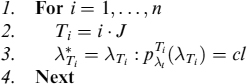
Having determined the levels of maximum default intensity, we can compute the term structure of (minimum) discount factors for the zero-spreads corresponding to those levels:
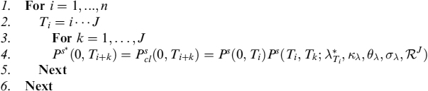
Armed with the minimum discount factors for each expiry, we can compute the total minimum discount factor for all expiries as:
for i = 1, …, N.
In building such curves we considered the cost of funding between two refunding dates as completely determined by the maximum ![]() at the beginning of the same period. In fact, there is no refunding risk and the curve is no different from that of deterministic spreads.
at the beginning of the same period. In fact, there is no refunding risk and the curve is no different from that of deterministic spreads.
The unexpected funding cost in (12.183), at a given confidence level, can now be readily computed for each period. To cover these unexpected costs the bank posts economic capital. At time Tdk the posted capital is:
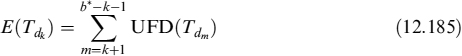
where b* ≤ b is the number of periods that the financial institution deems necessary to recapitalize the firm, should unexpected economic losses occur. The safest assumption is to set b* = b, so that the full economic capital needed up to expiry of the swap is taken into account. It is also true that market VaR is typically computed for a period of 1 year in banks, so that different choices can be adopted.
Assuming that the required economic capital is invested in risk-free assets, the annual premium rate π over the risk-free rate to remunerate it29 is a cost that the bank has to bear to cover unexpected funding costs. For simplicity's sake, without too great a loss of generality, let π be a constant; we thus have total funding cost given by the amount of debt left unpaid at the end of the swap, plus the present value of the annual premium paid on the economic capital for each period:

As above, FC is plugged into (12.172) to derive the fair swap rate, via a numerical search. The rate is once again the level making the present value of the funding cost FC = 0.
12.3.6 Including counterparty credit risk
Counterparty credit risk is a component of valuation that has not been considered up to this point. What is more, should the counterparty go bankrupt, then CVA should be included in the valuation.30
Let us assume that counterparty credit risk is nil for hedging swaps. This is not an unrealistic assumption as portfolio of hedging swaps is dealt with other banks, and they are provided with a CSA agreement that practically reduces expected losses to zero upon counterparty default.31 So we focus only on the effects that default of the main swap counterparty may produce on funding costs.
Let T be the time the counterparty of the swap defaults: if it occurs when the NPV of the swap is positive to the bank, then the latter will suffer a loss equal to NPV minus the recovery. This loss can be seen as the replacement cost the bank has to pay to re-enter a swap with the same contract terms as the one closed after the counterparty's default. The expected present value of this loss is simply the CVA, so the very fact of including it in the valuation at inception means the bank is basically receiving compensation for it. CVA can either be collected as a reserve or considered as a premium of an option and then hedged with market instruments, when available. In any case, the bank does not have to pay other costs when the counterparty goes bankrupt and the NPV is positive, since CVA covers their expected amount.
Let us now consider the case when the NPV of the swap is negative on counterparty default: the contract is closed out and its value has to be paid by the bank to the defaulting party. The amount needed for this payment can in theory be funded by reopening the same contract with another counterparty, under the hypothesis that the NPV paid to the defaulting party is the risk-free value of the contract and that the new contract is dealt with a default risk-free counterparty.32 In this case an upfront fee is paid to the bank by the new counterparty so as to compensate for the negative NPV and thus make the deal fair at inception. Nevertheless, it is easier for the bank to deal in par swaps quoted in the market and to fund with new debt the negative NPV to pay to the defaulting party.
Let us assume that counterparty default is the first jump of a Poisson process (with intensity λC) that can also be time dependent. We also assume it follows a CIR process such as bank default intensity. The probability of default between t and T is defined as:
Let TT be the first fixed leg payment date of the closed swap after default. Expected exposure at a certain time T is given by the expected negative value of the swap's NPV:
which is the difference between the original swap and the new par swap dealt in the market at TT and expiring at Tb. Let cf(TT) = ENE(t, T): this is a negative cash flow and has to be funded by the bank for payment of the NPV to the defaulting party: the funded amount is repaid using additional cash flows produced by the original portfolio of hedging swaps and the new swap struck at ST,b. At time Tcj, given the default at time T < Tcj, the cash flow is:
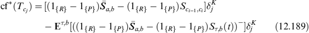
The first line in (12.189) is the same as when there is no default, whereas the second line is an additional cash flow, increasing (decreasing) the positive (negative) cash flows fixed before default, which can be used to repay the capital instalments of the debt. We define cfT(Tcj) as the additional cash flow such that the total new cash flow after default can be written as:
We are now in a position to generalize the two strategies explained above and determine the funding cost that includes the effects of counterparty risk.
More on Strategy 1: Funding all cash flows at inception
Let us assume we are computing funding costs implied by Strategy 1 in Section 12.3.4. For a default at T we need to find the additional amount of loan AT, with fixed interest rate ![]() and amortization schedule defined similarly to (12.169) (we use the same notation as above):
and amortization schedule defined similarly to (12.169) (we use the same notation as above):
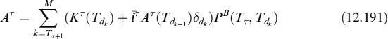
Available liquidity is defined as in (12.171) for given T, keeping in mind that it is created only if counterparty default occurs in the interval [TT−1, TT]. So, we weight it by the probability of default:
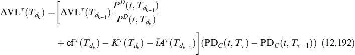
for Tdk−1 > TT, with AVLT(TT) = AT ≥ cf(TT) and K(Tdk) = cfT(Tdk).
Let us now consider the M possible defaults that may occur in the interval [Tdk−1, Tdk], at times Tm, with M ∈ {1, 2, …, M}. Total available liquidity is:

Total available liquidity must satisfy the same two conditions as when there is no counterparty risk. Funding cost FC is defined in exactly the same way as when there is no credit risk: it is the present value at time t of the amount the bank needs to add to the final instalment, not generated by the cash flow structure of the hedged deal, that allows it to fully repay the debt, keeping in mind the funding of the NPV that has to be paid to the defaulting party.
More on Strategy 2: First approach to compute unexpected funding costs
If Strategy 2 (Section 12.3.5) is adopted to compute funding costs, then we have to consider that at each possible default time an additional outflow has to be added to the rollover of the debt issued by the bank to finance negative cumulated cash flows, followed by additional inflows as defined in (12.189).
Let FDBT(Tk+1) be the amount of debt needed to fund the cash flows produced by default at T. Its expected evolution is given by:
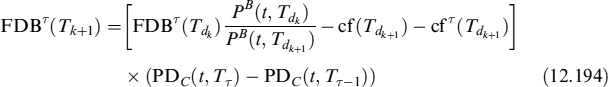
for Tdk−1 > TT, and FDBT(TT) = (TT).
The total debt rolled over is then:

where we use the same notation as above. The unexpected funding cost may be computed by either of the approaches sketched when there is no counterparty risk. Total funding cost is given by (12.181) or (12.186), with EFD(Tdk) = TFDB(Tdk).
Funding costs including counterparty default can be added to CVA to get:

A numerical search has to be operated in this case too so that fair swap rate Sa,b(0) can be retrieved.
12.3.7 Practical examples
We now show how the strategies described above can be practically implemented. We will price a market standard 10-year swap, with the fixed leg paying annually and the floating rate paying semiannually: both legs have a fixed notional amount equal to 100. To value the fair rate of this swap, without including any other adjustment due to counterparty risk and funding costs, we need the term structure of OIS and 6M Libor, from which we also derive the discount factors. We adopt the market practice of considering the OIS the best proxy for the risk-free rate in the interbank market. Table 12.15 shows these data.
The funding costs that the bank has to pay depend on the probability of default modelled in a reduced-form setting with a stochastic intensity whose parameters are shown in Table 12.16. The resulting spread discount bonds and total discount factors are given in Table 12.17, as are the forward funding spreads as defined in (12.176).
Given these market data, the fair swap rate can easily be derived; it is S0,10(0) = 3.3020%. Future cash flows of this swap can be hedged, as suggested above, using a portfolio of 1-year forward starting swaps (except the first one which is a 1-year spot starting swap); these swaps have to be market standard, in the sense that the fixed leg pays annually whereas the floating leg pays semiannually, in much the same way as the 10-year swap. In Table 12.18 we show the fair swap rate for each hedging swap for the year when the corresponding fixed leg pays. The floating leg of each hedging swap matches a portion on the floating leg of the 10-year swap. Assuming that the bank is a fixed rate receiver of the 10-year swap, net cash flows for the hedged position are shown in Table 12.18. In Figure 12.4 we show cumulated cash flows whose value, compounded at the risk-free rate, can be summed algebraically to zero.
From Table 12.18 we can check that the receiver swap, once hedged, does not imply any negative cumulated cash flow, so that the bank does not have to resort to any additional external funding. The fair swap rate for the bank is the same as above and no adjustments for funding costs need to be included. This does not mean that the CVA for counterparty credit risk and the DVA for its own default risk can be disregarded, despite doing so in the current analysis: this example demonstrates that DVA is not the funding cost for a derivative contract, in accordance with what we stated in Chapter 10.
Table 12.15. Term structures of OIS and 6M Libor forward rates and of the corresponding discount factors for both
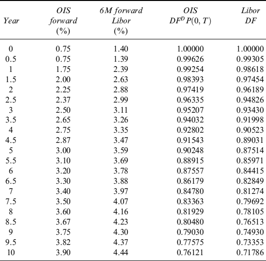
Table 12.16. Parameters of default intensity
| λ0 | 0.50% |
| κλ | 1.00 |
| θλ | 1.95% |
| σλ | 20.00% |
| R | 0% |
Let us now assume that the bank has a payer position in a 10-year swap: all cash flows with a positive (negative) sign in Table 12.18 should now be considered as paid (received), so that the compounded cumulated cash flow is always negative and nil at expiry. This is true if the bank is able to borrow money at the risk-free rate; since the bank can actually default with a positive probability, it pays a funding spread to borrow money. We analyse both strategies suggested above to cope with funding needs originated by negative cumulated cash flows and verify how the fair swap rate is modified.
Let us start with Strategy 1, which involves funding all negative cash flows at inception. Numerical search for the starting amount of the debt, subject to the constraints stated above, and for the fair swap rate that makes the present value of the funding cost FC zero are shown in Table 12.19. The fixed interest rate paid annually by the bank on the debt is 4.2761% and is obtained via (12.170). This rate applied to the debt oustanding at the beginning of the period yields the interest paid. Starting amount A that the bank has to borrow is 4.1746 and the amortization plan shown guarantees that it is fully repaid and that no available liquidity is left at expiry of the contract. The final fair swap rate is ![]() , a correction of around 6bps.
, a correction of around 6bps.
Table 12.17. Forward funding spreads and the term structures of spreads and total discount factors
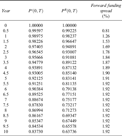
Let us now examine how Strategy 2 can be implemented: the bank borrows money when negative cash flows occur, if cumulated cash flows are negative, or the debt is rolled over in the future. The unexpected funding cost is measured in the first of the two approaches (i.e., by means of spread options). The results are shown in Table 12.20. Terminal outstanding debt is negative (i.e., there is cash inflow) and its present value compensates the sum of the present value of unexpected funding costs (last column), ![]() ; the final fair swap rate is
; the final fair swap rate is ![]() .
.
In Table 12.21 we present the results that would apply if the second approach were adopted to measure unexpected funding costs. Spread discount factors at a confidence level of 99% are computed using the procedure outlined above (they are shown in the last column). We assume a constant premium over the risk-free rate for the economic capital equal to π = 5%. Capital is posted to cover all future losses at any time until expiry of the contract, so that b* = b in formula (12.185). The fair swap rate (S0,10(0) = 3.2089%) is once again computed so that the total funding cost is nil. The terminal outstanding amount of the debt is negative, meaning that the bank has an inflow: the present value of a positive cash flow even in this case compensates the cost of the economic capital posted to cover unexpected funding losses, ![]() .
.
Table 12.18. Swap rates of hedging swaps and net single, cumulated and compounded cumulated cash flows for a hedged 10-year receiver swap
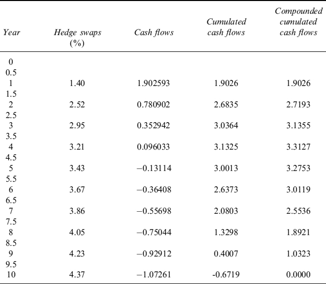
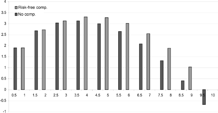
Figure 12.4. Compounded and non-compounded cumulated cash flows for a 10-year receiver swap
Table 12.19. Amount of outstanding debt, interest paid and available liquidity. Final values may be slightly different from zero due to the degree of approximation chosen in the numerical search (Strategy 1).
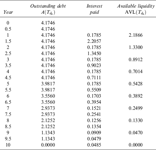
Finally, in Table 12.22 we summarize results to allow easy comparison amongst the different ways to include funding costs in the pricing of a swap. Given the term structure of interest rates and the probability of default, Strategy 1 (funding everything at inception) and Strategy 2 (unexpected finding costs measured with spread options) produce very similar results: the fair rate of a payer swap is abated by about 6 bps in both cases. Strategy 2, with unexpected costs measured at a given confidence level and covered by economic capital, is more expensive and the fair swap rate decreases by around 10 bps.
It is worthy of note that this relationship amongst the three adjustments may not hold in every case. It may well be for forward starting swaps (say, a 10Y5Y) that the first approach of Strategy 2 turns out to be more convenient than Strategy 1. In any case, the only hedging scheme that fully protects the bank is Strategy 1, since it also avoids exposure to future liquidity shortages. So, this risk should always be kept in mind despite it being very difficult to measure.
Table 12.20. Single and cumulated cash flows, debt rollover and present value of unexpected funding costs for each period measured using spread options. Final values may be slightly different from zero due to the degree of approximation chosen in the numerical search (Strategy 2, first approach).
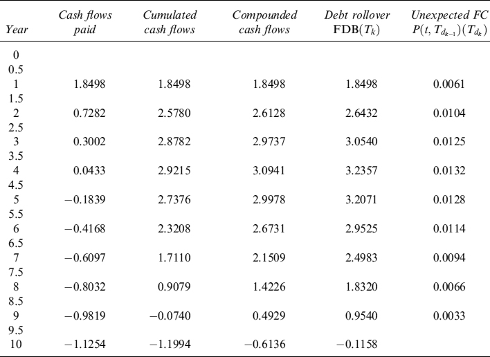
Table 12.21. Single and cumulated cash flows, debt rollover and present value of unexpected funding costs for each period, measured at a confidence level of 99%. Final values may be slightly different from zero due to the degree of approximation chosen in the numerical search (Strategy 2, second approach).
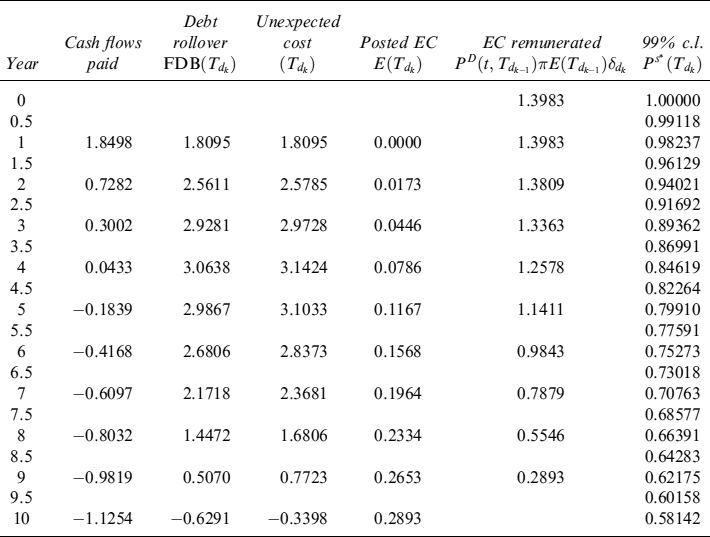
Table 12.22. Effects on the fair swap rate of including funding costs according to the different methods proposed
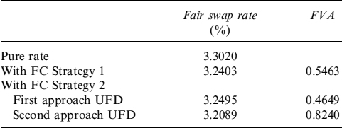
1 See Chapter 10 for the distinction between “price” and “value”.
2 Some CSA agreements allow rehypothecation of collateral, so the counterparty receiving collateral can actually freely use the cash (or the assets) it receives.
3 In fact, they take bilateral counterparty credit risk into account, as well as the cost of funding borne by each of the counterparties involved.
4 When γ < 100% (i.e., there is not full collateralization), then residual counterparty credit risk should be priced into the contract. To isolate the effect of collateral, we do not consider counterparty credit risk still present in the event of imperfect collateralization. The inclusion of counterparty credit risk in the pricing of derivative contracts, keeping the funding costs due to collateral management in mind, has been studied in [104], where arguably the most comprehensive pricing formula is presented.
5 This can easily be verified by setting γ = 0 in equation (12.6).
6 This example is the same as an example in [56], with the exception that our example includes a collateral agreement.
7 See Chapter 10 for a detailed discussion on this. For an alternative view, see [95].
8 We used 45 time steps within the contract's duration of 1 year and a 50-point Gauss–Legendre quadrature scheme for each time step.
9 Both the setup and the notation are the same as in [89].
10 We present an analysis of how funding costs should be included in a non-collateralized swap later on; the analysis here applies to the non-collateralized fraction of the contract (i.e., 100% − γ).
11 At a given confidence level c.l., we used the equation ![]() (where α is a point of the normal standard distribution returning probability c.l.) to determine the corresponding swap rate value at time T. In the example, c.l. = 99% implies that α ≈ 2.326.
(where α is a point of the normal standard distribution returning probability c.l.) to determine the corresponding swap rate value at time T. In the example, c.l. = 99% implies that α ≈ 2.326.
12 Units of domestic per foreign currency, so that XXX is the base and YYY is the numeraire currency.
13 A similar formula was derived in [69].
14 In practice, the bank will never be able to find a completely risk-free counterparty, but if the interest yielded by the bank account issued by the latter is fair, it should include remuneration for expected default losses, so that on a risk-adjusted basis net yield is still the risk-free rate.
15 Just the value – not the price – is risk-neutral. This means that an economic agent bearing the same costs to replicate the contract agrees on the value of the contract independently of its risk aversion. Replication, in the presence of funding and collateral costs, depends on the long or short position we wish to reproduce.
16 Note that the borrowing is collateralized in static fashion at the start of the contract (i.e., the amount of the currency one party pays against receiving an amount of the other currency). This static collateral is not readjusted daily as happens with a CSA agreement, so there is still the risk that, on counterparty default, the market value is unable to fully cover the loss suffered by the surviving party.
17 See [44] for details on FX market conventions.
19 This seems to be the standard when swaps are cleared via the LCH, since the collateral is always posted in USD. Although the collateralization process involves multilateral netting in this case, its mechanics are the same as in the bilateral CSA agreement and, hence, valuation of the contract can be operated in the same way.
20 For more details on the new pricing formulae that have been developed in the wake of the financial crisis of 2007 see [21] and [89].
23 See Chapter 10 for a discussion on this point.
24 As far as defaultable issuers are concerned, their debt should be remunerated by a spread over the risk-free rate to compensate for the risk of default so that, ultimately, expected return is still the risk-free rate.
25 See Chapter 10 for a more detailed discussion.
26 The forward risk survival measure uses the defaultable discount bond as a numeraire. For more details see [110]. We would like to stress that we are measuring funding costs under a going concern principle, which frees the bank from considering its own default in the evaluation process.
27 A non-central χ2 with d degrees of freedom and non-centrality parameter c is defined as function χ2(x; d, c).
28 The superscript t′ to the expectation operator E[·] means that we are working in the t′ forward risk-adjusted measure. Technically speaking, we are calculating expectations by using the bond Ps(0, t′) as a numeraire.
29 Basically, the ROE minus the risk-free rate.
30 Bilateral counterparty risk implies that DVA should also be included in the pricing during the bargaining process. Once the deal has been struck, DVA is simply a cost that the bank has to bear. On the differences between price and value and on the notion of DVA as a cost see Chapter 10.
31 The funding costs due to the collateralization of swap contracts can be included in the analysis using this approach.
32 For an analysis of the different closeout clauses see [36].