6.1 A TAXONOMY OF CASH FLOWS

The identification and taxonomy of the cash flows that can occur during the business activity of a financial institution is crucial to building effective tools to monitor and manage liquidity risk.

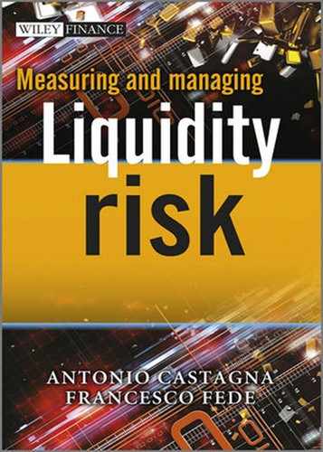
Many classifications have been proposed (see, amongst others, [86]; a good review is [107]). The taxonomy we suggest, not too different from the others just mentioned, focuses on two main dimensions: time and amount; it is sketched in Figure 6.1. Like any other classification, this one also depends on the reference point of view. More specifically, in our case, we classify cash flows by considering them from a certain point in time; for example, cash flows may fall in one of the categories we will present below when we look at them from, say, today's point of view of. They can also change category when we shift the point of view in some other date in the future.

The first dimension to look at, when trying to classify future cash flows, is time: cash flows may occur at future instants that are known with certainty at the reference time (e.g., today), or they may manifest themselves at some random instants in the future. In the first case we say that, according to the time of their appearance, they are deterministic. In the second case we define them as stochastic (again, according to time).

The second dimension to consider is the amount: cash flows may occur in an amount that is known with certainty at the reference time, or alternatively their amount cannot be fully determined. For the amount, the main distinction will be between deterministic cash flows, if they fall in the first case, or stochastic cash flows, if they belong to the second case. Classification according to the amount, though, can be further broken down such that subcategories can be identified.

Moreover, when the amount is deterministic, cash flows can be labelled simply as fixed as a result of being set in such a way by the terms of a contract.

When the amount is stochastic, it is possible to recognize four possible subcategories labelled as follows: credit related when amount uncertainty can be due to credit events, such as the default of one or more of the bank's clients; indexed/contingent, when the amount of cash flows depends on market variables, such as Libor fixings; behavioural, when cash flows are dependent on decisions made by the bank's clients or counterparties: these decisions can only be loosely predicted according to some rational behaviour based on market variables and sometimes they are based on information the bank does not have; and, finally, the fourth subcategory is termed new business: in which cash flows originated by new contracts that are dealt in the future and more or less planned by the bank, so that their amount is stochastic.

Based on the classification we have introduced, we can provide some examples of cash flows, with the corresponding category they belong to, according to the time/amount criterion. The examples are also shown in Figure 6.1.

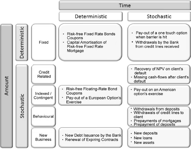
Figure 6.1. Taxonomy of the cash flows

Let us begin with deterministic amount/deterministic time cash flows: they are typically related to financial contracts, such as fixed rate bonds or fixed rate mortgages or loans. These cash flows are produced by payments of periodic interests (e.g., every six months) and periodic repayment of the capital instalments if the asset is amortizing. It should be noted that not only bonds or loans held in the assets of the bank generate these kinds of cash flows, but also bonds issued and loans received by the bank held in its liabilities. Moreover, when considering assets, that cash flows belong to the fixed amount/deterministic time category can only be ensured if the obligor, or the bond's issuer, is risk free, so that credit events cannot affect the cash flow schedule provided for in the contract.

Deterministic amount cash flows can also occur at stochastic times, either because the contract can provide for a given sum to be paid or received by the bank, or because the amount depends on a choice made by the bank. An example of the first kind of cash flow can be represented by the payout of one-touch options: in fact, the buyer of this type of option receives a given amount of money when the underlying asset breaches some barrier level, from below or from above. The time is unknown from the reference instant, but the amount can easily be deducted from the contract's terms. An example of cash flows that depend on the bank's decisions can be represented by the positive cash flows originated by the withdrawals of credit lines received by the bank. In this case, the amount can safely be assumed to be some level between 0 and the limit of the credit line chosen by the bank depending on its needs, but it can occur at any time until the expiry of the contract, since liquidity needs may arise at some stochastic time.

Shifting the analysis to the stochastic amount category, we first identify credit-related cash flows that are due to the default of one or more clients, so that once the default time is fixed, their amount can be implied. The default time is obviously not known at the reference time, so that the time when these cash flows occur is stochastic. An example can be represented by the missing cash flows, after the default, of the contract stream of fixed interests and of capital repayment of the loan. A missing cash flow may be considered a negative cash flow that alters a given cash flow schedule: if a loan, for example, is fixed rate amortizing, then we have a modified cash flow schedule on the contract interest rate and capital repayment times. Moreover, the recovery value after default can be inserted in this category of cash flows.

Stochastic amount cash flows we can also be indexed/contingent (i.e., linked to market variables). Examples of such cash flows are, amongst others, floating rate coupons that are linked to market fixings (e.g., Libor) and the payout of European options, which also depend on the level of the underlying asset at the expiry of the contract. In these the time of the occurrence of cash flows is known (the coupon payment, the exercise date), but there may also be indexed/contingent cash flows that can manifest at stochastic times. Examples are the payout of American options, both when the bank is long or short them, because the exercise time is stochastic and depends on future market conditions that determine the optimality of early exercise. Again, here we have to stress that we are referring to contracts whose counterparty to the bank is default risk free.

Another type of stochastic amount cash flow is behavioural; for example, when a bank's clients decide to prepay the outstanding amount of their loans or mortgages. In this case the bank may compute the prepaid amount received on prepayment: the prepayment time cannot be predicted with certainty by the bank, so that the time when the cash flows occur is stochastic in this case. Missing cash flows with respect to the contract schedule can be determined once prepayment occurs. If the prepaid mortgage, as before, is fixed rate amortizing, then we have a modified cash flow schedule on the contract interest rate and capital repayment times.

Other behavioural cash flows, befalling at stochastic times, are those originated by credit lines that are open to clients: withdrawals may occur at any time until the expiry of the contract and in an uncertain amount, although within the limits of the line. Withdrawals from sight or saving deposits belong to this category too.

Finally, we have stochastic amount cash flows related to the replacement of expiring contracts and to new business activity. For example, the bank may plan to deal new loans to replace exactly the amount of loans expiring in the next two years, and this will produce a stochastic amount of cash flows since it is unsure whether new clients will want or need to close such contracts. Old contracts expire at a known maturity so that cash flows linked to their replacement are known as well. Moreover, the new issuance of bonds by the bank can be well defined under a time perspective, but the amount may not be completely in line with the plans.

By the same reasoning, the evolution of completely new contracts may not follow the pattern predicted in business development documents, so that related cash flows are both amount and time stochastic. For example, new retail deposits, new mortgages and new assets in general may be only partially predicted. In general, cash flows due to new business, or to the rollover of existing business, are quite difficult to model and to manage.

6.2 LIQUIDITY OPTIONS

Some of the categories of cash flows described above are connected with the exercise of so-called liquidity options. These kinds of options are conceptually no different from other options, yet the decision to exercise them depends on their particular nature.

More specifically, a liquidity option can be defined as the right of a holder to receive cash from, or to give cash to, the bank at predefined times and terms. Exercising a liquidity option does not directly entail a profit or a loss in financial terms, rather it is as a result of a need for or a surplus of liquidity of the holder. This does not necessarily exclude linking the exercising of a liquidity option to financial effects; on the contrary, such a link is sometimes quite strong: this is clear from the examples of liquidity options we provide below.

Comparing these options with standard options usually traded in financial markets, the major difference is that the latter are exercised when there is a profit, independently of the cash flows following exercise, although typically they are positive. For example, a European option on a stock is a financial option that is exercised at expiry if the strike price of the underlying asset is lower than the market price. The profit can immediately be monetized by selling the stock in the market so that the holder receives a positive net cash flow equal to the difference between the strike price (paid) and the sell price (received). Alternatively, options may be exercised and the stock not immediately sold in the market, so that only a negative cash flow occurs: this is because the holder wants to keep the stock in her portfolio, for example, and it is more convenient to buy it at the strike price instead of the prevailing market price. The convenience to exercise is then independent of the cash flows after exercise.

On the other hand, a liquidity option is exercised because of the cash flows produced after exercise, even if it is sometimes not convenient to exercise it from a financial perspective. For example, consider the liquidity option that a bank sells to a customer when the bank opens a committed credit line: the obligor has the right to withdraw whatever amount up to the notional of the line whenever she wants under specified market conditions, typically a floating rate (say, 3-month Libor) plus a spread, that for the moment we consider determined only by the obligor's default risk. The option to withdraw can be exercised when it also makes sense under a financial perspective; for example, if the spread widened due to worsening of the obligor's credit standing: in this case funds can be received under the contract's conditions (which are kept fixed until expiry) and hence there is a clear saving of costs in terms of fewer paid interests on the line's usage rather than opening a new line. On the other hand, the line can be used even if the credit spread shrinks, so that it would be cheaper for the obligor to get new funds in the market with a new loan, but for reasons other than financial convenience it chooses to withdraw the needed amounts from the credit line.

Another example of a liquidity option is given by sight and saving deposits: the bank's clients can typically withdraw all or part of the deposited amount with no or short notice. The withdrawal might be due to the possibility to invest in assets with higher yields more than compensating for higher risks, or it might be due to the need of liquidity for transaction purposes. So, even in this case there may exist some financial rationale behind exercising a liquidity option, but it can also be triggered by many other different reasons that are hardly predictable, or can be forecast on a statistical basis.

Exercising a liquidity option can also work the other way round: the bank's client has the right to repay the funds before the contract ends. Although the bank would benefit in this case from the greater amount of liquidity available, economic effects are usually negative and thus cause a loss. An example is given by the prepayment of fixed rate mortgages or loans: they can be paid back before the expiry for exogenous reasons, often linked to events in the life of the client such as divorces or retirements; more often prepayment is triggered by a financial incentive to close the contract and reopen it under current market conditions if the interest rate falls. In the first case the bank would not suffer any loss if market rates rose or stayed constant, on the contrary it could even reinvest at better market conditions those funds received earlier than expected. In the second case, prepayment would cause a loss since replacement of the mortgage or closure of the the loan before maturity would be at rates lower than those provided for by old contracts.

In the end, although liquidity options can be triggered by factors other than financial convenience, the effect on the bank can be considered twofold:

1. A liquidity impact on the balance sheet, given by the amount withdrawn or repaid.
2. A (positive or negative) financial impact, given by the difference between the contract's interest rates and credit spread and the market level of the same variables at the time the liquidity option is exercised, applied on the withdrawn or repaid amount.

Sometimes the second impact is quite small, as, for example, when a client closes a savings account: the bank's financial loss is given in this case by the missing margin between the contract deposit rate and the rate it earns on the reinvestment of received amounts (usually considered risk-free assets), or by the cost to replace the deposit with a new one that yields a higher rate. The liquidity impact, on the other hand, can be quite substantial if the deposit has a big notional.

While the financial effects of liquidity options can be directly, although partially, hedged by a mixture of standard and statistical techniques, the liquidity impact can only be managed by the tools that we analyse in the following. These tools, loosely speaking, involve either cash reserves or a constrained allocation of the assets in liquid assets or easy access to credit lines (i.e., a long position in liquidity options for the bank). All of these imply costs that have to be properly accounted for when pricing contracts to deal with clients, so that models to price long and short liquidity options have also to be designed. Since, as shown above, liquidity options also produce financial profits or losses when exercised, so that they can also be seen under some respects as financial options, models must jointly consider liquidity and financial aspects.

6.3 LIQUIDITY RISK

Risk is always related to uncertainty about the future: this may turn out to be more favourable than initially expected or, on the contrary, more adverse than forecast. Although positive and negative outcomes should be balanced, in practice it is the adverse unexpected states of the world that is of interest. Bearing this in mind, a very general definition of liquidity risk for a financial institution is the following.

Definition 6.3.1 (Liquidity risk). The event that in the future the bank receives smaller than expected amounts of cash flows to meet its payment obligations.

We have already analysed the different kinds of liquidity concepts and related risks in Chapter 2. Definition 6.3.1 encompasses both funding liquidity risk and market liquidity risk. In fact, if a bank is not able to fund its future payment obligations because it is receiving less funds than expected from clients, from the sale of assets, from the interbank market or from the central bank, this risk may produce an insolvency situation if the bank is absolutely unable to settle its obligations, even by resorting to very costly alternatives. Market liquidity risk according to the definition above is the result of the inability to sell assets, such as bonds, at fair price and with immediacy, and leads to a situation in which the bank receives smaller than expected amounts of positive cash flows.

The risk dimension considered in Definition 6.3.1 refers to the quantity of flows, so we call this quantitative liquidity risk. Nonetheless, we claim that another risk dimension for liquidity should be considered: the cost of liquidity, or cost of funding, and the related risk can be defined as follows.

Definition 6.3.2 (Funding cost risk). The event that in the future the bank has to pay greater than expected cost (spread) above the risk-free rate to receive funds from sources of liquidity that are available.

This can be defined as cost of liquidity risk or cost of funding risk. Not too much attention has been paid to the modelling of funding cost risk, although in the past it was always recognized as such but deemed to have little impact on banking activity. The reason for this is quite simple to understand if one looks at Figure 6.2, which shows the rolling series of the CDS Itraxx Financial spread. We use this as a proxy for funding spread over the risk-free curve for top European banks on a 5-year maturity. As is manifest, the spread was almost constant and low until 2007 (the outbreak of the subprime crises in the US). This means that banks were considered virtually default risk free and funding costs, meant as the spread over the risk-free curve, had a very limited effect on the profitability of banks.

Moreover, it should be stressed that in such a constant low-spread environment, the rollover of the bank's liabilities that expire entails negligible risk in terms of unexpected spread levels. This combined with abundant liquidity such that the quantity of funding available was in practice without relevant limits, banks were able to decide how to finance their assets as they preferred: the rollover of maturity was an almost risk-free activity. For these reasons, trying to predict funding costs was a futile exercise and their inclusion in the pricing of contracts was straightforward.

Since the middle of 2007, financial institutions have no longer been able to always raise funds at low spreads: the volatility of spreads even over interbank market rates (e.g., Libor) dramatically increased, and the amount of funding available in the capital market declined, at least for the banking sector. As a consequence of these two reasons, the funding policy of banks is now subject to constraints so as to abate the average funding cost, reduce rollover risk (regarding both the quantitative and risk dimension) and hence make credit intermediation activity still a profitable business.

Figure 6.2. CDS Itraxx Financial rolling series from September 2004 to September 2011

Source: Market quotes from major brokers

The conclusion we can draw from this is that modern liquidity risk management must consider both the quantitative dimension and the cost dimension as equally important and robust modelling must be developed for the two dimensions. We can synthesize both dimensions of liquidity risk in the following comprehensive definition.

Definition 6.3.3 (Liquidity risk). The amount of economic losses due to the fact that on a given date the algebraic sum of positive and negative cash flows and of existing cash available at that date, is different from some (desired) expected level.

This definition includes a manifestation of liquidity risk as:

1. Inability to raise enough funds to meet payment obligations, so that the bank is forced to sell its assets, thus causing costs related to the non-fair level at which they are sold or to suboptimal asset allocation. The complete inability to raise funds would eventually produce an insolvency state for the bank. These costs refer to the quantitative dimension of liquidity risk.
2. Ability to raise funds only at costs above those expected. These costs refer to the cost dimension of liquidity risk.
3. Ability to invest excess liquidity only at rates below those expected. We are in the opposite situation to point 2, and it is a rarer risk for a bank since business activity usually hinges on assets with longer durations than liabilities. These (opportunity) costs also refer to the cost dimension of liquidity risk.

6.4 QUANTITATIVE LIQUIDITY RISK MEASURES

We introduce a set of measures to monitor and manage quantitative liquidity risk.¹ These measures aim at monitoring the net cash flows that a bank might expect to receive or pay in the future and ensure that it stays solvent. Cash flows, however, classified according to the taxonomy above are produced by two classes of factors.

Definition 6.4.1 (Causes of liquidity). All factors referring to existing and forecast future contracts originated by the ordinary business activity of a financial institution can be considered as the causes of liquidity risk. Cash flows generated by the causes of liquidity can be both positive and negative.

The other class of factors is given by Definition 6.4.2.

Definition 6.4.2 (Sources of liquidity). All factors capable of generating positive cash flows to manage and hedge liquidity risk and can be disposed of promptly by the bank determine the liquidity generation capacity (defined in the following) of the financial institution.

First we set the notation. Let us indicate with the sum of expected positive cash flows occurring at time t_i from the reference time t₀. Similarly, we indicate by the sum of expected negative cash flows occurring on the same date.

We analysed above the different categories of cash flows and saw that many are stochastic in terms of the amount or time of occurrence or both. This is the reason we have stressed the fact that the sum of cash flows, either positive or negative, is just expected. On the other hand, if cash flows are expected, this also means that their distribution at each time should be determined so as to recover measures other than the expected (average) amount, to increase the effectiveness of liquidity management. We will come back to this later on, but for the moment we can formally define the positive and negative cash flows for the set of contracts and/or securities {d₁, d₂,…, d_N as:

and similarly

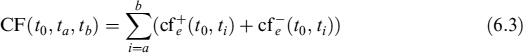
Assume we are at the reference time t₀: we define by CF(t₀, t_j) the cumulative amount of all cash flows starting from date t_a up to time t_b:

Expected cash flows and cumulated cash flows allow us to construct the basic tools for liquidity monitoring and management: the term structure of expected cash flows.

6.4.1 The term structure of expected cash flows and the term structure of expected cumulated cash flows

The term structure of expected cash flows (TSECF) can be defined as the collection, ordered by date, of positive and expected cash flows, up to expiry referring to the contract with the longest maturity, say t_b:

At the end of the TSECF, with an indefinite expiry corresponding to the end of business activity, there is reimbursement of the equity to stockholders. TSECF is often referred to as the maturity ladder: we reserve this name for the initial part, up to one-year maturity, of the TSECF. It is also standard practice to identify short-term liquidity, up to one year, and structural liquidity, beyond one year.

The term structure of cumulated expected cash flows (TSECCF) is similar to the TSECF: it is the collection of expected cumulated cash flows, starting at t₀ and ending at t_b, ordered by date:

The TSECCF is useful because banks are interested not only in monitoring the net balance of cash flows on a given date, but also how the past dynamic evolution of net cash flows affects its total cash position on that date. If on a given date the balance of inflows and outflows is net negative, this position can be netted out with a positive cash position originated by past inflows. Obviously the reverse can also be true and the bank can use a net positive inflow on a given date to cover a short cash position deriving from past outflows, although in this case it should be noted that short cash positions must be financed in any case, typically with new liabilities (see below), so that positive inflows are used to pay back these debts.

Conceptually, building the TSECF and TSECCF is quite simple and can be shown with an example.

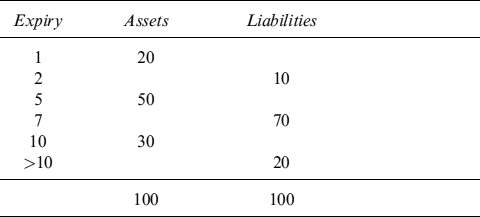
Example 6.4.1. Consider a bank with a simplified balance sheet like the one in Figure 6.3. The assets comprise investments in bonds and loans; they are financed with deposits, bonds and equity. Assume that the assets bear no default risk and no liquidity options are embedded within deposits. The first step to build the TSECF is to order the assets and the liabilities according to their maturity, disregarding which kind of contract they are. This is shown in Table 6.1.

When assets expire positive cash flows are received by the bank, whereas when liabilities expire negative cash flows must be paid by the bank. The amount of the cash flows is simply the notional of each contract in the assets and liabilities and, under the assumptions we are working with, these amounts are deterministic both under a time and amount perspective. Collecting them and ordering them by date, we obtain the TSECF in Figure 6.4.

Cash flows in themselves are not enough to monitor the liquidity of a bank, since what matters in the end is the cash available up to a given time, which is given by the cumulated cash flows. At each date, cash flows from the initial date t₀ up to each date t_i are cumulated according to formula (6.3) and entered in the TSECCF: the result is also shown in Figure 6.4.

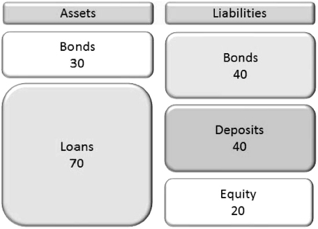
Figure 6.3. Balance sheet of a bank with types of assets and liabilities and their quantities.

Table 6.1. Assets and liabilities reclassified according to maturity

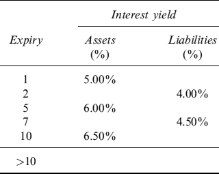
This overly simplified example can be made a bit more realistic if we also consider the interest payments that assets and liabilities yield. Assume a yearly period for coupon payments and an average yield common to all contracts expiring on a given date: the interest yielded by each contract is shown in Table 6.2.

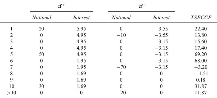
When interest payments are added, the TSECF is built as in Table 6.3, where there is also the TSECCF. In Figure 6.5 the TSECF is represented for each date, decomposed in positive and negative cash flows, and in the bottom diagram cumulated cash flows are also shown.

In Example 6.4.1 shows a very simple balance sheet producing a very simple TSECF and related TSECCF. In a real balance sheet the number and type of contracts entering into the analysis is much greater and is not just limited to those existent at the reference time, but also all new activities that can be reasonably expected to be operated and in most of cases belonging to the category of new business of Figure 6.1.

In greater detail, the cash flows of the TSECF are those produced by all the causes of cash flows, as defined above. This means that the TSECF

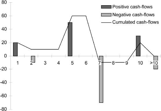
Figure 6.4. Term structure of expected cash flows for the simplified balance sheet reclassified in Table 6.1

Table 6.2. Interest yield of the assets and liabilities of the simplified balance sheet reclassified in Table 6.1

• includes the cash flows from all existing contracts that comprise the assets and liabilities: in many cases cash flows are stochastic because they can be linked to market indices, such as Libor or Euribor fixings (interest rate models are needed to compute expected cash flows);
• cash flows are adjusted to consider credit risks: credit models have to be used to take into account defaults on an aggregated basis by also considering the correlation existing amongst the bank's counterparties;
• cash flows are adjusted to account for liquidity options: behavioural models are used for typical banking products such as sight deposits, credit line usage and prepayment of mortgages;

Table 6.3. The term structure of cash flows and of cumulated cash flows

• cash flows originated by new business increasing the assets should be included: they are typically stochastic in both the amount and time dimensions, so they are treated by means of models that consider all related risks;
• the rollover of maturing liabilities, by similar or different contracts, and new bond issuances (which could also be included in the new business category) to fund the increase in assets, have to be taken into account. The risks related to the stochastic nature of these flows have to be properly measured as well resulting in a need to set up proper liquidity buffers and we will dwell on that in Chapter 7.

The TSECF, and hence the TSECCF, do not include the flows produced by the sources of cash flows, which we analyse below. The sources of cash flows are tools to manage the liquidity risk originated by the causes of cash flows.

The task of the Treasury Department is to monitor the TSECF and the TSECCF. The perfect condition is reached if the TSECCF is positive at all times. This means that positive cash flows are able to cover negative cash flows, both of which are generated by usual business activity. Although this is the ideal situation it cannot be verified for two reasons:

1. Many of the cash flows belong to categories that are stochastic in the amount and/or the time dimension, such that the TSECF always forecasts just the expected value of a distribution of flows. As a result the TSECCF contains only expected values as well: if it is positive on average most of the time, the distribution of cumulated cash flows at a given time can also actually envisage negative outcomes with an assigned probability.
2. The temporal distribution of the maturities of the assets and the liabilities could produce periods of negative cumulated cash flows. These periods may be accepted if they are short and can be managed effectively with the tools we introduce below.

When the TSECCF shows negative values, on an expected basis, this means that the bank may become insolvent and eventually go bankrupt. This is why the treasurer's main task is to ensure that the future TSECCF is always positive. But since we have seen that this ideal situation cannot always be fulfilled, we need to discover which tools can be used to cope with the case when the TSECCF has negative values.

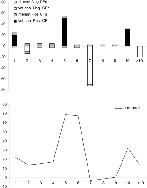
Figure 6.5. Term structure of expected cash flows for the simplified balance sheet reclassified in Table 6.1 including interest payments (top) and term structure of expected cumulated cash flows (bottom)

6.4.2 Liquidity generation capacity

Liquidity generation capacity (LGC) is the main tool a bank can use to handle the negative entries of the TSECCF. It can be defined as follows.

Definition 6.4.3 (Liquidity generation capacity). The ability of a bank to generate positive cash flows, beyond contractual ones, from the sources of liquidity available in the balance sheet and off' the balance sheet at a given date.

The LGC manifests itself in two ways:

1. Balance sheet expansion with secured or unsecured funding.
2. Balance sheet shrinkage by selling assets.

Balance sheet expansion can be achieved via

• borrowing through an increase of deposits, typically in the interbank market (retail or wholesale unsecured funding);
• withdrawal of credit lines the financial institution has been granted by other financial counterparties (wholesale unsecured funding);
• issuance of new bonds (wholesale and retail unsecured funding).

It is worth noting that new debt is not the same as that planned to roll over existing contracts or to fund new business: in this case the related cash flows would be included in the TSECF and in the TSECCF, as seen above.

Balance sheet shrinkage is operated by selling assets, starting from more liquid ones such as Treasury bonds, corporate bonds and stocks: they are traded in the market actively and can be sold within a relatively short period. Reduction may also include the sale of less liquid assets, such as loans or even buildings owned by the bank, within a more extended time horizon.

Repo transactions can also be considered separately from the other cases and labelled as “balance sheet neutral”.

The bank may prefer to consider only liquidity that can be generated without relying on external factors, such as clients or other institutional counterparties. It is easy to recognize that LGC related to balance sheet expansion is dependent on these external factors, whereas balance sheet reduction, or “balance sheet neutral” repo transactions, are not. So it is possible to present an alternative distinction within LGC; namely, we can identify

• balance sheet liquidity (BSL), or liquidity that can be generated by the assets existing in the balance sheet. BSL is tightly linked to balance sheet reduction LGC and it is also the ground on which to build liquidity buffers, which we will analyse in Chapter 7;
• remaining liquidity, originated by the other possible ways mentioned above, which relates to balance sheet expansion.

A similar classification within LGC is based on the link between the generation of liquidity and the assets in the balance sheet, so that we have:

• Security-linked liquidity including
  • secured withdrawals of credit lines received from other financial institutions;
  • secured debt issuance;
  • selling of assets and repo.
• Security-unlinked liquidity including
  • unsecured borrowing from new clients through new deposits;
  • withdrawals of credit lines received from other financial institutions;
  • unsecured bond issuance;

It is immediate clear that security-linked liquidity is little more than BSL liquidity, or the liquidity obtained by balance sheet reduction.

To sum up, we can identify three types of sources of liquidity that can be included in the classifications above:

1. Selling of assets, AS.
2. Secured funding using assets as collateral and via repo transactions, RP.
3. Unsecured funding via withdrawals of committed credit lines available from other financial institutions and via deposit transactions in the interbank market, USF.

The first two sources generate security-linked BSL by reducing the balance sheet or keeping it constant. The third source generates security-unlinked non-BSL by expanding the balance sheet. It is worth stressing that the unsecured funding of point 3 is not the same as the unsecured funding we inserted in the TSECF and TSECCF, but is mainly related to the rollover of existing liabilities or the issuance of new debt to finance business expansion. In fact, while in the latter case we referred to existing and planned activity funding usual banking activity, the operations involved in LGC refer to shorter term exceptional unsecured funding, in most cases unrelated to a bank's bond issuance and other forms of fundraising.

We can now define the term structure of LGC as the collection, at reference time t₀, of liquidity that can be generated at a given time t_i, by the sources of liquidity, up to a terminal time t_b:

where AS(t₀, t_i) is the liquidity that can be generated by the sale of assets at time t_i, computed at the reference time t₀; RP(t₀, t_i) and USF(t₀, t₁) are defined similarly.

Analogously, the term structure of cumulated LGC is the collection, at the reference time t₀, of the cumulated liquidity that can be generated at a given time t_i, by the sources of liquidity, up to a terminal time t_b:

Remark 6.4.1. The quantities entering in the TSLGC and hence the TSCLGC are expected values, since they all depend on stochastic variables such as the price of assets and the haircut applied to repo transactions. Moreover, the stochasticity of the amount of unsecured funding that it is possible to raise in the market could and should be considered.

The sources of liquidity contributing to the TSLGC belong either to the banking or the trading book. In the banking book the sources of liquidity are all the bonds available for sale² (AFS) and other assets that can be sold and/or repoed relatively easily: they are referred to collectively as eligible assets. In all cases these assets are unencumbered; that is, they are not already pledged to other forms of secured funding such as the ones we present just below. To determine at a given date t_i the liquidity that can be generated by these sources, one needs:

• AFS bonds: the expected future value of each bond, considering the volatility of interest rates and credit spreads, and of the probability of default. Moreover, the possibility that the bonds may become more illiquid, thus increasing bid–ask spreads and lowering the selling price, has to be considered in the analysis.
• For other assets the selling period and the expected selling price have to be properly taken into account.

As mentioned above, assets in the banking book can be also repoed; that is, the bank can sell them via a repo transaction and buy them back at expiry of the contract. The repo can be seen as a collateralized loan that the bank may receive: as such it can be safely assumed that liquidity can be obtained more easily than unsecured funding, since the credit risk of the bank is considerably abated. For the same reason the funding cost, meant as the spread over the risk-free rate, is also dramatically reduced for the bank.

Besides the factors that affect liquidity that AFS bonds can generate, there is another factor determining the actual liquidity that can be obtained by a repo or a collateralized loan transaction: the haircut, or the cut in the market value of the bond indicating how much the counterparty is willing to lend to the bank, given an amount of bonds transferred as collateral. The haircut will depend on the volatility of the price of the collateral bond and on the probability of default of the issuer of the bond.

Haircuts have to be modelled not only for unencumbered assets to assert their liquidity potential, but also for encumbered assets, involved in collateralized loans, to forecast possible margin calls and reintegration of the collateral when their prices decline by an appreciable amount.

Finally, received committed credit lines, which are not exactly in the balance sheet until they are used (in which case they become liabilities) have to be included in the TSLGC and their amount and future actual existence taken into account. In fact, although it is also quite reasonable to receive committed credit lines from other financial institutions after the expiry of the lines currently received, their amount could be constrained by possible systemic liquidity issues. Moreover, the costs in terms of funding spreads and other fees to be paid have to be considered as well.

If we move to the trading book, we can identify bonds and other assets similar to those included in the banking book as sources of liquidity. Amongst the other assets that can be used to generate liquidity we may add stocks and also some structured products, such as eligible ABSs or even more complex structures.³ These assets, provided they are unencumbered, can be sold or they can be pledged in collateralized loans or repoed. In these cases the same considerations we have made above can be repeated here and the same factors have to be included in the assessment of the liquidity potential to include in the TSLGC.

Unsecured funding on the interbank market via deposit transactions, usually up to one-year expiry, are part of the banking book for accounting reasons. Also here, the possibility to resort to this source of liquidity should be carefully weighted by the possibility to experience systemic liquidity crises (e.g., as in 2008) that strongly limit the availability of funds via this channel. The other important factor is the costs related to the funding spread.

Building the TSLGC can be very difficult, since the assumptions made for a given period affect other periods. For example, if the bank wants to compute the liquidity-generating capacity provided by a given bond held in the assets, assuming it is pledged as collateral for a loan starting in t₁ and expiring in t₂ to cover negative cumulated cash flows occurring during the same period, then the same bond has to be excluded for the same period and other overlapping periods from the TSLGC. This means that the process to build the actual TSLGC should be carried out in a greater number of steps.

It should also be stressed that the TSLGC is intertwined with the TSECF (and thus the TSECCF): there are feedback effects when defining the TSLGC that affect expected cash flows. which makes the building process a recursive procedure to be repeated until an equilibrium point is reached. For example, if we still consider that the TSLGC for a given period can be fed by a bond that can be pledged as collateral or repoed, then the cash flows of this bond should be excluded from the TSECF for the period of the loan or repo contract.⁴ Missing cash-flows for the corresponding period worsen the cash flow term structure (although marginally), but this means that they must also be included in the analysis.

In the end, most of the problems in building the TSLGC are caused by unencumbered assets (most of which are what we earlier referred to as AFS bonds), both because the bank must keep track of how many are either sold or repoed out, and because the liquidity amount that can be extracted from these assets depends on several risk factors. It is useful then to introduce a tool that helps monitoring this part of the LGC more thoroughly: it is the term structure of available assets (TSAA) and will be described in the next section.

6.4.3 The term structure of available assets

In the previous section we stressed that BSL is originated by selling assets and/or by the repo transactions made on them. When building the TSLGC, it is important to ascertain whether BSL is the result of setting assets or carrying out repo transactions, since both operations have different consequences in terms of liquidity.

When an asset, such as a bond, is purchased by a bank a corresponding outflow equal to the (dirty) price is recorded in the cash position of the bank. During the life of the bond coupon flows are received by the bank and finally, at expiry, the face value of the bond is reimbursed by the issuer. All these cash flows should be considered contract related, so that they are included in the TSECF and the TSECCF. The likelihood of the issuer defaulting should also be taken into account.

The TSAA is affected by purchases, since it records increases in the security for the amount bought. When the asset expires, the TSAA records a reduction to zero of its availability, since it no longer exists. During the life of the asset, the availability is affected by total or partial selling of the position, and by repo transactions.

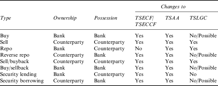
The TSAA is also affected by other kinds of transactions that can be loosely likened to repo agreements, but have different impacts. Namely, we also have to analyse buy/sellback (and sell/buyback) transactions and security lending (and borrowing). What matters in terms of availability for liquidity purposes is the possession of the asset rather than its ownership. We summarize all possible cases in the following:

• Repo transactions: at the start of the agreement the bank receives cash for an amount equal to the price of the asset reduced by the haircut; at the same time it delivers the asset to the counterparty. Although the asset is still owned by the bank, its possession passes to the counterparty, so that the bank no longer has availability of the security. This will become encumbered and cannot either be sold or used as collateral until the end of the repo agreement, when it is returned. Payments by the asset during the repo agreement belong to the bank since it is the owner, so that the TSECF and in the TSECCF are not affected in any way. The TSAA of the asset is reduced by an amount equal to the notional of the repo agreement, whereas the cash flow received by the bank at the start and the negative cash flow at the end are both entered in the TSLGC. Repo transactions produce a liability in the balance sheet, since they can be seen as collateralized debts of the bank.
• Reverse repo transactions: at the start of the agreement the bank pays cash for an amount equal to the price of the asset reduced by the haircut and receives the asset. The asset is owned by the counterparty, but it is now in the possession of the bank, so that it can be used as collateral by the bank for other transactions until the end of the repo agreement, when the obligation that it is to be returned to the counteparty has to be honoured by the bank. The payments by the asset during the repo agreement belong to the counterparty, so that they do not enter the TSECF or the TSECCF, but we include the cash flow paid by the bank at the start and the cash flow received at the end as contract, but only once. The TSAA of the asset is increased by an amount equal to the notional of the repo agreement. The TSLGC is not affected but the asset can be repoed until the end, so that it can be altered until this date. Reverse repo transactions are treated as assets in the balance sheet, since they can be seen as collataralized loans to the counterparty.
• Sell/buyback transactions: similar to repo transactions in terms of the exchange of cash and of the asset, with the difference that ownership passes to the buyer (the counterparty) at the start of the contract together with the possession. All payments received for the asset before the buyback belong to the counterparty.⁵ The cash flows between the start and end of the contract will be taken from the TSECF and the TSECCF. The TSAA of the asset decreases by an amount equal to the notional of the sell/buyback contract. The TSLGC is affected in the same way as in the repo agreement, since sell/buyback transactions are a way to generate BSL. Sell/buyback transactions represent a commitment for the bank at the end of the contract.
• Buy/sellback transactions: similar to reverse repo transactions in terms of the exchange of cash and of the asset, with the difference that ownership passes to the buyer (the bank) at the start of the agreement together with the possession. This implies that the payments received for the asset before the sellback belong to the bank, so that they enter the TSECF and the TSECCF, along with the cash flows at the start and end that relate to the purchase and sale, since they are contract flows. The TSAA of the asset is increased by an amount equal to the notional of the buy/sellback agreement. The TSLGC is not affected but the asset can be repoed until the end, so that it can be altered until this date. Buy/sellback transactions represent an asset for the period of the contract.
• Security lending: similar to sell/buyback transactions in terms of exchange of the asset, but no cash is paid by the counterparty to the bank (except a periodic fee as service remuneration). Only possession passes to the counterparty, so that the payments received for the asset before the end of the contract belong to the bank and they enter the TSECF and the TSECCF, as does the interest paid by the countertparty at expiry when returning the asset to the bank. The TSAA of the asset decreases by an amount equal to the notional of the lending, since the bank cannot use it as collateral or sell it. The TSLGC is not affected and the asset cannot produce any liquidity until the end of the contract. Security lending represents an asset of the bank for the period of the contract.
• Security borrowing: similar to buy/sellback transactions in terms of exchange of the asset, but no cash is paid by the bank to the counterparty (except a periodic fee as service remuneration). Possession passes to the bank, so that the payments received for the asset before the end of the contract belong to the counterparty. The TSECF and the TSECCF are not affected apart from the interest paid by the bank at expiry of the borrowing. The TSAA of the asset increases by an amount equal to the notional of the borrowing, since the bank can use it as collateral provided it returns it to the counterparty at expiry. The TSLGC is not affected but the asset can produce liquidity until the end of the contract. Security borrowing represents a liability of the bank.

Other assets, such as stocks, do not have a specific expiry date. In this case contract cash flows entering the TSECF and the TSECCF are just the initial outflow representing the price paid to purchase the asset and the periodic dividend received. Moreover, non-maturing assets can be the underlying of repo transactions, buy/sellback (sell/buyback) contracts and security lending (and borrowing): the analysis is the same as above.

In Table 6.4 we recapitulate the results for all types of contracts that can be written on assets. It is worth noting that TSLGC is always affected either because the contract is dealt to generate BSL or because LGC is potentially increased over its lifetime. The only contract that does not increase the TSLGC is security lending, which actually decreases LGC related to BSL.

The TSAA can now be built keeping these results in mind, since for a given asset it is defined as the collection, for each date from an initial time t₀ to a terminal date t_b, of the quantity in possession of the bank, regardless of its ownership. In fact, the main purpose of the TSAA is to indicate how much of the asset can be used to extract liquidity and thus its contribution to global LGC. In more formal terms, for an asset A₁ we have:

where is the quantity of the asset in possession of the bank at time t_i. On an aggregated basis, regarding a set of M securities in possession of the bank, the total TSAA including all the assets is:

Table 6.4. Types of contracts involving assets and effects on the TSECF/TSECCF, TSAA and TSLGC.

The TSAA only shows how many single securities, or all of them, are available for inclusion in LGC. Obviously, this does not imply that the notional amount can be fully converted into liquidity. According to the type of operation (selling or repo) the price and/or the haircut are factors that need to be considered to determine the actual amount of liquidity that can be generated. Hence, we need proper models that allow the bank to forecast expected (or stressed) values for the price and the haircut, both at the single and aggregated assets level: such models will be introduced in Chapter 7 when we discuss the liquidity potential of a buffer comprising bonds.

In Example 6.4.2 we show how the interrelations amongst the different term structures operate in practice.

Example 6.4.2. The bank buys a bond at time 0 for a notional amount of 1,000,000 at a price of 98.50; the payment is settled after 3 days, when the bond's possession also passes to the bank. In Table 6.5 we show what happens to the term structures. The bond pays a semiannual coupon of 10% p.a. and it expires in 2 years.

The TSECF records an outflow equal to the notional amount of the bond times the price (we assume the bank buys the bond upon a coupon payment, so that the dirty price and the clean price are the same) occurring on the settlement date, 3 days after the reference time 0 (or 0.01 years). The TSAA records an increase of the quantity available to the bank of the bond until its expiry, when it is reset to zero. The TSLGC is unaffected. The last two columns show the price and the haircut. They are expected values and for the moment we consider them as given, although they can be the output of some model or just assumptions of the bank.

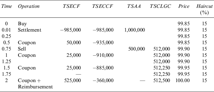
Assume now the bank decides to sell a quantity of the bond equal to a notional of 500,000 after 9 months (or 0.75 years). We know that this trade can be dealt to generate liquidity, so that the TSCLGC records an inflow equal to the amount times the price, including the accrued interests (500,000 × (99.90/100 + 10% × 0.25) = 512,000 as well. The TSECF and the TSECCF are modified so as to show the reduced amounts of interest and capital received on the scheduled dates. The TSAA records a cut in the available amount for 500,000 until expiry of the bond, when it drops to zero. Table 6.6 shows the results.

Table 6.5. Purchase of a bond: effects on term structures

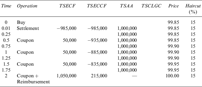
Table 6.6. Selling of a bond: effects on term structures

Let us now analyse the effects of repo and reverse repo transactions on term structures. Assume the bank repoes the bond after 3 months (0.25 years) for a notional amount equal to 500,000 and a period of 6 months. Given the price and the haircut of the bond, and keeping accrued interest in mind, the amount of cash received by the bank is:

500,000 × (99.85% + 10% × 0.25) × (1 − 15%) = 424,469

In Table 6.7 the TSCLGC indicates an increase of liquidity, whereas the TSAA indicates that the available quantity of the bond dropped to 500,000.

The bank pays 9% as interest on this repo transaction, so that the terminal price paid when getting the bond back is:

424,469 × (1 + 9% × 0.5) = 443,569.84

The difference 443,569.84 − 424,469 = 19,101.09 should be considered as a contract cash flow so that it enters the TSECF on the date at the end of the repo. The TSCLGC drops to zero and the TSAA returns the available amount back to 1,000,000.

Table 6.7. Repo and reverse repo of a bond: effects on term structures

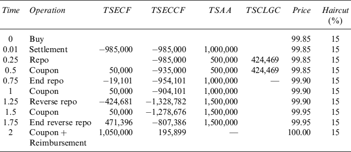
After 1 year and 3 months (1.25 years) the bank deals a 6-month reverse repo on this bond for a notional of 500,000. The price it pays to deliver the bond at inception is

500,000 × (99.90% + 10% × 0.25) × (1 − 15%) = −424,681

This amount enters the TSECF and alters the TSECCF as a consequence; what is more, the TSAA increases up to 1,500,000 since the bond is in possession of the bank. All this is shown in Table 6.7. The TSCLGC is left unchanged.

At the end of the reverse repo contract, assuming the interest rate paid by the counterparty is 11%, the inflow received by the bank is:

424,681 × (1 + 11% × 0.5) = 471,396

which should be considered fully as a contract cash flow, thus entering the TSECF; the bond is returned to the counterparty and consequently the TSAA is set back to 1,000,000 as shown in Table 6.7.

When the bank operates buy/sellback (or sell/buyback) operations, the effects are different. Assume that after 3 months (0.25 years) the bank buys 400,000 bonds and sells it back after 6 months at the forward price. At the start of the contract the bank pays:

400,000 × (99.85% + 10% × 0.25) = 409,400

This sum enters the TSECF and the quantity of the bond available increases to 1,400,000 in the TSAA. The TSCLGC is not modified by this operation. During the lifetime of the contract the bank is the legal owner of the bond and receives all the payments as well.

At the end of the contract (0.75 years) the bank sells the bond back at the contract price, typically the forward price prevailing at the inception of the contract (which we assume equal to the predicted price 99.90). The sum it receives also includes accrued interest:⁶

400,000 × (99.90% + 10% × 0.25) = 409,600

Table 6.8. Buy/sellback and sell/buyback of a bond: effects on term structures

This sum also enters the TSECF, while the TSAA shows a reduction of the available quantity back to 1,000,000. All this is shown in Table 6.8.

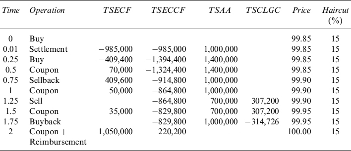
In Table 6.8 we also show the effects of a sell/buyback of the bond starting after 1 year and 3 months (1.25 years) and terminating after 6 months (1.75 years). The price received by the bank is:

300,000 × (99.90% + 10% × 0.25) = 307,200

which is included in the TSCLGC since the operation can be seen as a way to extract BSL from the available assets; the TSAA indicates a reduction of the available quantity down to 700,000. At the end of the contract the bank buys the bond back and pays:

300,000 × (99.95% + 10% × 0.25) = 314,726

which is included in the TSCLGC. The TSAA increases back to 1,000,000. The coupon paid during the life of the contract is proportional to the available quantity of 700,000.

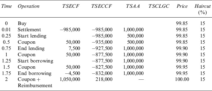
We now show what happens to the different term structures when a security lending and borrowing is operated by the bank. Let us start with a case in which the bank lends 500,000 of the bond after 3 months for a period of 6 months. The TSECF does not record any cash flow at the inception of the contract, whereas the TSAA shows a reduction of the available quantity of 500,000. After 6 months the bond is returned to the bank (the TSAA increase) and the bank receives a fee for the lending, which we assume equal to 3% p.a.:

500,000 × (3% × 0.5) = 7,500

The coupon paid during the lifetime of the contract are possessed by the legal owner (i.e., the bank). This can be observed in Table 6.9.

The bank borrows a quantity of 300,000 of the same bond at 1.25 years for a period of 6 months. The TSAA is only affected at the start and end of the contract. The TSECF only records the borrowing fee paid by the bank:

300,000 × (3% × 0.5) = 4,500

Table 6.9. Lending and borrowing of a bond: effects on term structures

6.5 THE TERM STRUCTURE OF EXPECTED LIQUIDITY

The term structure of expected liquidity (TSL_e) is basically a combination of the TSECCF and the TSLGC. Formally, it can be written as:

where we have included the term TSECCF(t₀, t₀): although it may seem strange, it is simply the cash existing at the initial time in the balance sheet, so that:

TSECCF(t₀, t₀) = Cash(t₀)

The TSL_e is in practice a measure to check whether the financial institution is able to cover negative cumulated cash flows at any time in the future, calculated at the reference date t₀.

If the Treasury Department aims at preserving a positive sign for the TSECCF for all maturities, and this cannot always be guaranteed, as soon as we add it to our analysis of the TSCLGC we end up with a total picture for projected expected liquidity and the means the financial institution has at its disposal to cover negative cumulated cash flows (i.e., the TSL). The TSL must always be positive if the financial institution has to be solvent all the time. The TSL_e includes all possible expected cash flows generated by ordinary business activity, new business, the liquidity policy operated and the measures taken to cope with negative cumulated cash flows. If in the end it is impossible to exclude negative expected cumulated cash flows, then it is also impossible to prevent the financial institution from becoming insolvent.

Example 6.5.1. Let us revert back to Example 6.4.1 and expand it to take account of the TSAA and the TSCLGC with the objective of finally building a TSL_e. The main results are shown in Table 6.10.

Table 6.10. The term structure of expected liquidity and its building blocks

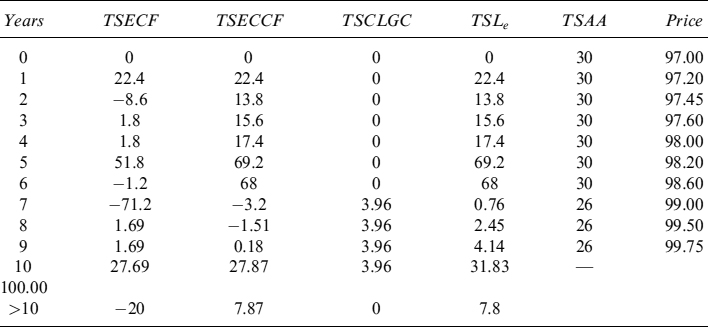
First, we start with the TSECF and the TSECCF of Table 6.3 of Example 6.4.1: the TSECCF is negative between the 7th and 8th year. This negative cumulated cash flow must be covered and in the balance sheet there is a bond that can be sold to create (BSL) liquidity. In fact, in Table 6.10 the TSAA includes an amount for the bond equal to 30 until the 6th year, then in the 7th year an amount of 4 is sold at the (expected) price of 99.00, so as to generate a liquidity of 3.96, which is included in the TSCLGC thereafter.

It should be noted that selling the bonds affects the TSECF, and hence the TSECCF, in the two ways shown in the previous section: there are fewer inflows for interest paid by the bond and the final reimbursement is lower as well. In this example the change in the TSECF does not produce other negative cumulated cash flows, so the LGC can be limited to selling the bond.

The TSL_e is the sum of the TSECCF and the TSCLGC at each period as shown in Table 6.10: it is always greater than or equal to zero, so the bank is in (expected) liquidity equilibrium. Figure 6.6 shows how the TSECCF, the TSCLGC and the TSL_e have evolved: the first and the last term structure clash on the same line until the seventh year, when the TSECCF becomes negative and it has to be counterbalanced by the TSCLGC.

6.6 CASH FLOWS AT RISK AND THE TERM STRUCTURE OF LIQUIDITY AT RISK

Section 6.1 discussed a taxonomy of cash flows according to the time and amount of their occurrence, most cash flows are stochastic in either or both dimensions. This is the reason we introduced the term structure of expected cash flows, cumulated cash flows and expected liquidity generation capacity: they flow into the term structure of expected liquidity which represents the main monitoring tool of a Treasury Department.

Nonetheless, the fact that cash flows are stochastic suggests that not only one synthetic metric of the distribution (i.e., the expected value) should be taken into account, but also some other measure related to its volatility. In this way it is possible to build the same term structure we analysed above from a different perspective showing the extreme values that both positive and negative cash flows may assume during the time of their occurrence.

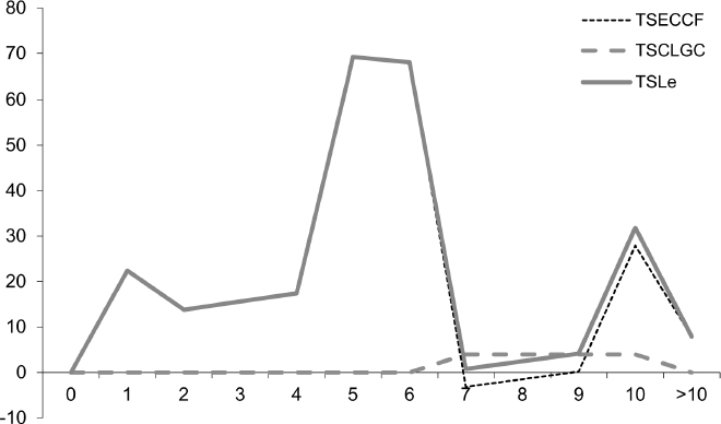
Figure 6.6. Term structure of expected cumulated cash flows, of cumulated liquidity generation capacity and of expected liquidity

In order to achieve this result, we need to link the single cash flows originated by contracts on and off the balance sheet to risk factors related to market, credit and behavioural variables. A number of approaches are described in Chapters 8 and 9. Here we show the general principles to build term structures that we define as unexpected with respect to the expected ones we looked at earlier.

The first concept to introduce is the positive cash-flow-at-risk, defined as

On a given date t_i, determined by the reference date t₀, the maximum positive cash flow, computed at a given confidence level , is reduced by an amount equal to the expected amount of the (sum of positive and negative) cash flows on the same date (cf_e(t₀, t_i; x)). It is worthy of note that we have added a dependency of the cash flows on x: this is an array x = [x₁, x₂,…, x_R] of R risk factors, which include market, credit and behavioural variables.

Analogously, a negative cash-flow-at-risk is defined as:

where in this case on a given date t_i, determined by the reference date t₀, the minimum negative cash flow, computed at a given confidence level , is netted with the expected cash flow occurring on the same date (cf_e(t₀, t_i; x)).

Note that the distribution of cash flows ranges from the smallest, possibly but not necessarily, negative ones to the largest, possibly but not necessarily, positive ones. Given a confidence level of α, on the right-hand side of the distribution all cash flows bigger than , whose total probability of occurrence is 1 − α, are neglected. In the same way, on the left-hand side of the distribution all cash flows smaller than , whose total probability of occurrence is still 1 − α, are not taken into account.

Once we have defined the cfaR, it is straightforward to introduce the term structure of unexpected positive cash flows, given a confidence level of α. This is the collection of positive cfaR for all the dates included between the start and the end of the observation period:

Similarly, the term structure of unexpected negative cash flows, given a confidence level of 1 − α, is:

The and can be described as the upper and lower bound of the term structure of cash flows, centred around the expected level that is given by the TSECF. It does not make much sense to build a cumulated and , since they will rapidly diverge upward or downward at unreasonable levels without providing accurate information for liquidity risk management. It is much more useful to build a term structure of unexpected liquidity that includes both the term structure of cash flows and liquidity generation capacity jointly computed at some confidence level α. We will dwell on that below; but first we give an example of and .

Example 6.6.1. We present a simplified TSCF and TSECF for a set of fixed and floating cash flows for a period covering 14 days. The notional amount for each date and for each type of index is shown in Table 6.11. For example, on the first day a contract of 1,000,000 produces an outflow indexed to 1-month Libor: it could be a bond the bank issued. There are also some dates when cash flows are not indexed to a floating rate, such as Libor, but have a fixed rate.

Table 6.11. Notional amount indexed to different Libor fixings and fixed cash flows, for cash flows occurring in a period of 20 days

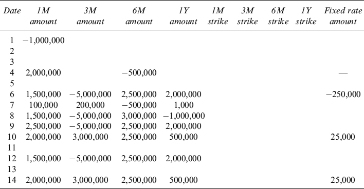
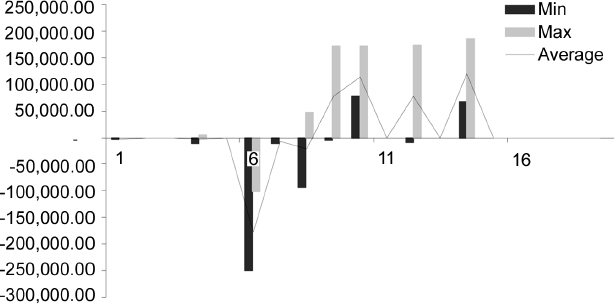
Figure 6.7. Maximum, minimum (at the α = 99% c.l.) and expected (average) cash flows for a period of 20 days.

We simulate 10,000 scenarios with a stochastic model for the evolution of the interest rate: the Cox, Ingersoll and Ross model (CIR, [54]), which will be analysed in greater details in Chapter 8.⁷ Each simulation allows different fixing levels for each date to be computed, then correspondingly we can determine the TSCF. For each date we will have 10,000 possible cash flows that are ordered from the lowest to the highest. We choose a confidence level α = 99%, which lets us identify the minimum cash flow as the 100th and the maximum cash flow as the 9,900th in the ordered set of cash flows for the 14 days. Moreover, we compute the expected level on each date, which is simply the average of the 10,000 possible cash flows. The result is shown in Figure 6.7. It is worthy of note that the minimum cash flow is not necessarily an outflow (i.e., a negative number).

To ascertain the impact of possible derivative features on the TSCF, we now introduce some caps at different strike levels for the last two dates (as shown in Table 6.12). In this case, if the index rate to which the cash flows are linked fixes higher than the cap's strike level the level is always considered equal to the strike.

The results are shown in Figure 6.8: they are derived in the same way as above but they take the caps into account as well. Compared with the results in Figure 6.7, it is easy to see that caps have the effect of lowering the maximum cash flow and reducing the expected (average) level as well. The effects are not unequivocally predictable, they depend on the strike level, the notional amount and the buying or selling of the optionality. In any case a simulation is needed to verify the distribution of cash flows for a given period.

As anticipated before setting out Example 6.6.1, it makes little sense to construct a TSL-at-risk simply as the sum of the TSCCF and the TSCLGC computed separately at a given confidence level. In fact, if we try to build a maximum or a minimum TSCCF by summing the items that comprise the TSCF_α or the TSCF_1−α, we would end up with extreme term structures that would look rather unlikely in practice, unless some dramatic event really happens. This is explained by the fact that negative cash flows, although calculated at their minimum at the chosen confidence level, are actually netted by the LGC that is forecast at its maximum at the same confidence level. So, negative cash flows do not really cumulate at extreme values, when considered at the all-encompassing balance sheet level. While it is possible from a mathematical point of view, and meaningful from a risk management point of view, to build the TSECCF and the expected TSCLGC separately and then sum them together in the TSL_e, it is mathematically wrong and managerially misleading to sum two term structures computed separately at extreme levels.

Table 6.12. Notional amount indexed to different Libor fixings and fixed cash flows, for cash flows occurring in a period of 14 days, with some cash flows capped

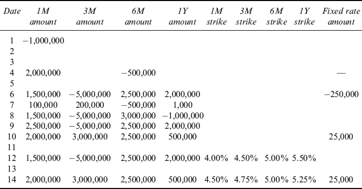
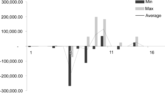
Figure 6.8. Maximum, minimum (at the α = 99% c.l.) and expected (average) cash flows for a period of 20 days, with some cash flows capped.

From these considerations, we need to calculate at an aggregated level the net cash flows included in both the TSCF and the TSLGC. To this end we can use the following procedure.

Procedure 6.6.1. The steps to compute aggregated cash flows and their maxima and minima are:

1. Simulate a number N of possible paths for all the R risk factors of the array x = [x₁, x₂,…, x_R]; each path contains M steps referring to as many calendar dates.
2. For each scenario n ∈ {1,…, N}, the cash flows included in the TSCF and the TSLGC are algebraically summed for each of M steps: we obtain a matrix N × M of aggregated cash flows:

   

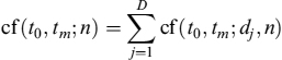
   where {d₁, d₂,…, d_D} are all the contracts and/or securities generating cash flows at date t_m, included in the TSCF and the TSLGC, under scenario n.

3. At each step m ∈ {1,…, M}, the maximum and minimum cash flows, at a confidence level of α and 1 − α, respectively, are identified. We denote them as cf_α(t₀, t_m) and cf_1−α(t₀, t_m), respectively.

Let us now define the TSL at the maximum and minimum extremes. In fact, the TSL with maximum cash flows at confidence level α is simply the collection of maximum cash flows derived using Procedure 6.6.1:

with the initial condition that TSL_α(t₀, t₀) = Cash(t₀). Similarly, the TSL with minimum cash flows at confidence level 1 − α is:

The two term structures of liquidity that we have just defined, together with the term structure of expected liquidity TSL_e, allow us to define a term structure of liquidity-at-risk (TSLaR): this is a collection of unexpected cash flows at each date in a given period [t₀, t_b], calculated as the difference between the minimum and the average level of cash flows. Although it is possible to compute the TSLaR for both the unexpected maximum and minimum levels, for risk management purposes it is more sensible to refer to the minimum unexpected levels, since unexpected inflows should not bring about problems. Then we formally define the TSLaR, at a confidence level of 1 − α, as:

It is easy to check, by inspecting formulae (6.15) and (6.10), that each element of the TSLaR_1−α is the difference between corresponding elements of the TSL_1−α and the TSL_e.

We have already mentioned that the curves presented in this section have to be computed by simulating the risk factors affecting all the cash flows at a balance sheet level. Stochastic models describing the evolution of risk factors are presented in the following chapters. Although their use is generally restricted to simulation engines to generate the TSL_e and the TSL_1−α, they can be used at a less general level to:

• calculate single metrics of interest, such as the TSAA of a single bond or of a portfolio of bonds, the TSLGC of the liquidity buffer (i.e., the fraction of LGC that relates to BSL);
• compute specific measure for one or more securities, such as haircuts and adjustments due to a lack of liquidity in their dealing in the market;
• measure single phenomena such as prepayments, usage of credit lines or the evolution of non-maturing liabilities (e.g., sight deposits);
• price the liquidity risk embedded in banking and trading book products.

When used independently the information derived by the models is useful for pricing and risk management, with the caveat that we are getting away from the more general picture where correlation effects play a big role. Thus, results obtained in this way should never form the basis for aggregation into a comprehensive measure of liquidity risk.

In the following chapters we present models that allow the bank to simulate the cash flows of the main items on its balance sheet and to build all the metrics we have described. But before doing so, we have to spend more time considering the liquidity buffer and term structure of funding liquidity and the interrelations existing between them when the bank plans an equilibrium liquidity policy.