10.1 INTRODUCTION

In this chapter we clarify the connections between funding costs and adjustments due to the compensation that a party has to pay to the counterparty for losses on a contract caused by its default (so-called debit value adjustment, hereafter DVA). We offer a robust conceptual framework so that DVA can be consistently included in the balance sheet of a financial institution.¹

Under the perspective we present below, DVA does not manifest any counterintuitive effects, such as reduction of the current value of the liabilities of a counterparty when its creditworthiness worsens. Moreover, identifying the link between funding costs and DVA, and the contribution of the credit risk the bank bears (so-called credit value adjustment, CVA) allows us to establish a method to discount positive and negative future cash flows thoroughly. The results are quite convenient since, after taking everything into account, things surprisingly and dramatically simplify, at least from a pricing and valuation point of view.

10.2 THE AXIOM

To derive a consistent theory of the links between funding and liquidity costs and counterparty and credit risks, we need to devise an axiom that will be both sensible and widely accepted.

Axiom 10.2.1. As in every human economic activity (by the very definition of the adjective “economic”), the stockholders of a bank aim at making profits out of their investments in business activity. As such they evaluate projects on the basis of the profits, costs and the expected profit margin to be shared at the end of the bank's activity.

The axiom assumes that the evaluators of the bank's investments are the shareholders. In reality, it is more likely that the evaluators are the managers of the bank, but nonetheless this does not impair the statement in the axiom since, to properly evaluate the profitability of investments, managers should do so as if they were shareholders. In fact, when a project is profitable for shareholders, it will also be profitable for all other creditors of the bank with a lower priority of claim on the bank's assets, if remuneration for each component of the entire capital structure is taken into account.

The end of bank activity can be indefinite such that profits are shared periodically: this is what usually happens in reality, where profits are computed and distributed on an annual basis. Alternatively, the end of bank activity can be voluntarily set at a given date.

It is worthy of note that default is not included in the definition of the voluntary end of activity, although the definition does not exclude the fact that default can be a rational option under some circumstances. In this case the decision to declare bankruptcy aims at minimizing losses and not at sharing (hopefully maximized) profits that are absent as a result of default.

Axiom 10.2.1 is sometimes referred to as a going-concern principle.²

10.3 CASH FLOW FAIR VALUES AND DISCOUNTING

We start by considering a simple loan contract (e.g., a term deposit in the interbank market). Assume there are two economic operators (e.g., two banks), B and L, the first of which would like to borrow money from the second. To keep things simple, let us assume that there exists a constant risk-free interest rate r and that each operator pays a funding spread s_X, X ∈ {B, L}, over the the risk-free rate when borrowing money.

The funding spread can be decomposed into two parts: (i) a premium that is required by the lender for the default probability of the borrower (indicated by π_X) and loss given default L_GDx (expressed as a fraction of the lent amount), and (ii) a possible liquidity premium γ_X (we still have X ∈ {B, L}).

At time t = 0, operator B asks operator L for a loan the amount of which returned at maturity T is K. L wants to price the risks and costs born in the contract, so as to make it fair (we assume that L does not want to earn any profit margin from the entire operation) and then to determine the amount P_L that can be lent, which makes the contract fair at inception. The present value of K at time T is its discounted value at rate r if counterparty B survives, but if B goes bankrupt, it is the present value of recovery (1 − L_GDX)K; to further lighten the notation, we assume without much loss of generality that L_GD = 100%, so that recovery is 0. We assume for the moment that γ_X = 0, so that S_X = π_X for either parties.³ We will relax both assumptions later on.

We have to sum the present value of the costs⁴ lender L has to pay: L has to fund the amount P and the future funding cost is the difference between the amount he has to pay back P_Le^(r+sL)T and the same amount invested at the risk-free rate P_Le^rT.⁵ Summing up these components, we get that the amount P_L that L can lend to B at time 0 can be obtained by making the value of the deal V_L at inception nil:

The fair amount lent will then be P_L = Ke^{−(r+sL+πB)T}, or

since we assumed the liquidity premium equal to 0.

Apparently, L has to discount the positive cash flows received at T at a discount rate that includes the risk-free rate, its own funding spread and the borrower's funding spread. Actually, this is an effective rate that can be used to determine the fair amount to lend, but it is more useful, in our opinion, to consider the discount rate as just the risk-free rate, and then use this to discount expected cash flows and costs. In fact, it is interesting to rewrite (10.1) in the following way:

where CVA_B = e^−rTKE[1 − 1_{TB > T}] is the credit value adjustment due to the loss given default of B, in this case equal to the entire amount times the probability of default; FC_L = e^−rTP_L(e^(r+sL)T − e^rT) is the funding cost borne by the lender. The fair amount P_L is easily recognized as the present value received at T, minus expected losses on default and minus funding costs: e^−rTK − CVA_B − FC_L.

In some works,⁶ funding costs take into account the probability of default of L: when the lender goes bankrupt, she will not return the compounded amount P to the funder, so that

Under the current assumption that γ^L = 0, funding costs would then be nil.

In our setting, given Axiom 10.2.1, it is not possible for the lender to consider her own default. Moreover, we honestly believe that it is very unlikely for the bank's management to argue in the presence of stockholders that they do not have to worry about not transferring funding costs in the pricing of their loans, because they will make up for all these extra costs when the bank goes bust. In fact, it is true that the bank will repay only a fraction (or nothing) of its debt on default, but this is a false saving of money, since not fully paying back debt obligation simply means that no equity is left to cover losses. So, saving on the repayment of the debt should more correctly be seen as a loss on shareholder equity. This will be clearer in what follows.

Let us now see how borrower B prices the loan contract. Basically, she evaluates the contract using the same principles as the lender, so that the fair amount P_B that she should receive should equal the present value of K, plus the funding costs and CVA_L for the losses suffered if the lender declares bankruptcy. In a loan contract CVA_L is zero, since the borrower has no exposure to the lender, but only an obligation. So we can write:

The fair amount to B is then P_B = Ke^−(r+sB)T, which is different from the amount fair to the lender. The latter also includes lenders' funding costs, whereas they are not considered in the valuation process by the borrower. What is more, it seems that negative cash flows should be discounted at an effective rate equal to the risk-free rate plus the borrower's spread, but this is just one way to set the fair level of the borrowed amount. Actually, it is more consistent, in our view, to use just one rate, the risk-free one, to discount expected cash flows and costs. In fact, recalling that γ^B = 0, we can write (10.3) as:

and hence P_B = e^−rTK − DVA_B, where DVA_B = CVA_B = e^−rTK(1 − e^−πBT) is debit value adjustment, or the expected loss the borrower will cause the lender in the event of her default. In a loan contract, DVA_B can also be seen as FC_B, or the funding cost the borrower has to pay: we will dwell more on this later on.

It is easy to check that P_B − P_L = FC_L. This means that no agreement can be reached by the two counterparties in the loan contract, since the fair amount the borrower requires is higher than what the lender is willing to lend. In other words, the borrower's fair amount does not include the lender's funding costs.

While this may come as a surprise, actually it is not so far from what has really happened in the last few years, starting in 2007, when bank funding spreads dramatically increased and the ability to close loan deals with counterparties worsened. Indeed, if the borrower has easy access to the capital market and she is able to ask for funds directly from investors, intermediation of the banking system is neither required nor efficient. Investors are economic operators investing their capital without (or with small) leverage, so that they do not include funding costs in their evaluation process. In this case it is possible to have an investor fair value that clashes with the borrower fair value, since they will only consider CVA_B = DVA_B in their capital allocation decisions.

An agreement can be reached between a lender who operates with funding (e.g., a bank) and a borrower only if the latter does not have direct access to the capital market, so that she will consider the lender's funding cost as unavoidable. In this case P_L = P_B.

The main result of this section is that the choice of discounting rate for positive and negative cash flows poses no problems even when there is a default risk premium and funding costs, when these are taken into account in a consistent manner. Actually, the discounting rate is only ever the risk-free rate. It is used to discount expected cash flows, expected losses given counterparty default and funding costs. Using effective discount rates (given by the sum of the risk-free rate, the credit spread and, where needed, the funding spread) in calculating the fair amount of a loan deal is misleading: the focus should not be on identifying the right discount rate for different cases, but on identifying expected cash flows and costs that may occur during the duration of the contract.

Following this route we totally bypass choosing the discount rate. Some people introduce a hedging argument for future cash flows and then consistently derive proper discount rates.⁷ We think that the proposed argument does not take into account the fact that each cash flow is not some abstract entity in the books of a financial institution, requiring a hedging strategy whose costs entail a specific discount rate. Cash flows, instead, are always originated within a specific contract, which implies there are costs, revenues and risks. These must be accounted for to calculate the value of the contract, and cash flows related to them have to be discounted with the risk-free rate. Incidentally, note that the attribute “risk free” is quite superfluous here and it is only used since in practice (and often also in theory) effective rates are introduced that encompass many risks. For the sake of rigor, there is only one (possibly stochastic) interest rate that makes it possible to determine how much one unit of the numeraire good (i.e., money) is worth at future times.

10.4 CRITIQUE OF DEBIT VALUE ADJUSTMENT

A great debate is currently ongoing over debit value adjustment and its treatment in bank balance sheets. In this section we will endeavour to analyse what DVA really means, by looking at it from an accounting perspective as well, since we believe it adds to understanding of the issue.

We assume that borrower B is a bank with a very simplified balance sheet that is marked to the market.⁸ Mark to market is operated by discounting all expected and risk-adjusted cash flows at risk free rate r, as shown in the previous section. The stockholders decide to start activity with equity E and to stop it after a period of time T; amount E is deposited in bank account D₁, which we assume risk free; moreover, they require no premium over the risk-free rate, so that it is also the hurdle rate to value investment projects. We also assume that no liquidity premium is paid by the borrower so that s^B = π^B.

10.4.1 Single-period case

Time 0

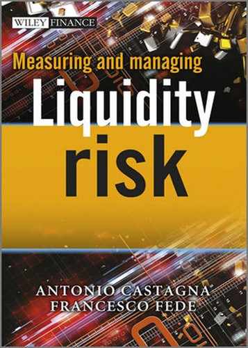
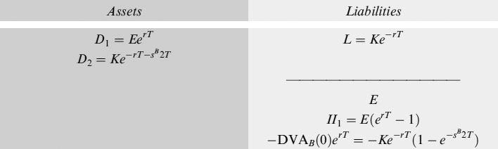
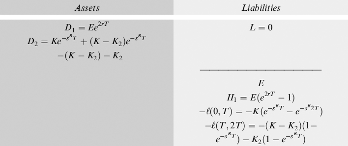
At time 0, the bank closes a loan contract with a lender (e.g., an institutional investor) which is not charging any funding cost when setting the fair amount to lend. The amount is deposited in bank account D₂, also risk-free to avoid immaterial complications at the moment. The balance sheet at time 0 looks as follows:

The assets and liabilities balance and DVA_B(0) is deducted from the risk-free present value of the loan paying back K at T: in this way the present value of the loan matches exactly the amount of cash deposited in D₂, so that the deal generates no P&L (profits/losses) at inception.

Subtracting DVA from the current value of the risk-free present value of liabilities is generally how debit value adjustment is included in the balance sheet; this common practice brings the rather disturbing consequence that when the creditworthiness of B worsens (i.e., π^B (= s^B in our case) increases), the present value of liabilities declines: something counterintuitive that has been justified by several arguments that are not particularly convincing. Some banks in the last few years benefitted from this situation given the current concept of DVA, basically seen simply as CVA which the counterparty prices in the contract, considered from the obligor's perspective. We believe instead that, given Axiom 10.2.1, DVA is something different, as we hope to completely prove in what follows.

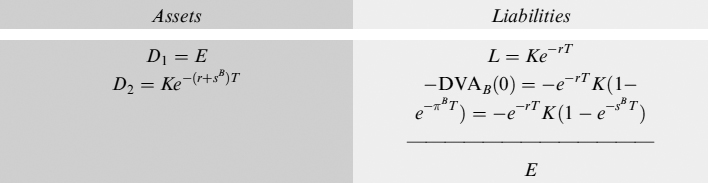
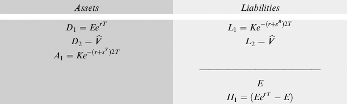
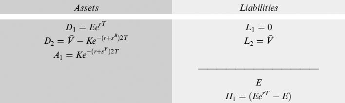
We suggest that DVA is not a reduction in the value of liabilities due to the credit risk of the borrower, but is actually the present value of the costs (or losses, if you wish) that the borrower has to pay due to the fact that he is not a risk-free economic operator, under Axiom 10.2.1. When DVA is considered as the negative of CVA, it still keeps its notion of compensation for counterparty risk, but this notion is only valid for the lender. Looking at it from the borrower's perspective, the negative of CVA (i.e., DVA) modifies its nature from that of compensation for a risk to that of a cost. Justifying the deduction from liabilities because of the compensatory nature of DVA, in light of Axiom 10.2.1, cannot be supported since stockholders do not consider their bank's default in the investment evaluation process. If this holds true, DVA, being a cost, should appear on the balance sheet to reduce the value of net equity, rather than the risk-free present value of the debt, so that the balance sheet should read:

The assets and liabilities still balance but now we have a completely different picture of the balance sheet, since the deal produces a P&L at inception: a loss equal to DVA. We now have to prove that DVA is actually the present value of the costs borne by the borrower until the expiry of the loan and the end of borrower activity.

Time T

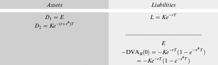
Let us check what happens at time T: all bank accounts earn the risk-free rate and this is also true for the risk-free value of debt; DVA(T) collapses to 0, since the debt expires. Eventually, we have:

The balance sheet clearly does not balance since we are missing the profits and losses realized over the period [0, T]. In fact, we have interest income from account D₁ (II₁) and losses on the funding spread given by the difference between what is the final value of D₂ and what is paid back on the loan:

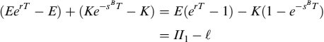
so that if we also add profits and losses to equity E and consider the outflow of cash to pay back the loan, the assets and liabilities balance again:

Lender activity is then closed and we value its profitability by also including the hurdle rate:

so that the entire activity generated a loss equal to the funding spread on amount K.

The terminal balance sheet also confirms the correctness of our suggestion to consider DVA as the value of the losses suffered at the end of the loan rather than a reduction of the risk-free present value of the loan. In fact, it is easy to check that realized losses are the compounded DVA: .

10.4.2 Multi-period case

Time 0

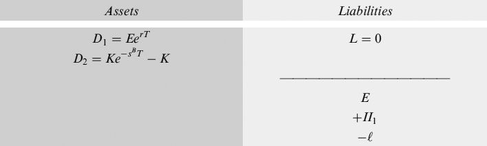
We would now like to generalize the analysis to a multi-period setting, by assuming that the bank's activity spans over the interval [0, 2T] made of 2 periods T: we will strike a balance in 0, at an intermediate time T and at the end of the activity 2T. We have the same setup as above and this time the bank asks for a loan maturing in 2T, when it has to pay back the amount K. The balance sheet at time 0 is:

DVA(0) is now the present value of the costs paid at 2T. They reduce the value of the equity E, following our definition of debit value adjustment.

Time T

At time T interest accrues on the bank accounts and on the loan. The interest earned on D₁ is II₁ = E(e^rT − 1); on D₂ the interest is II₂ = Ke^−SB2T(e^−rT − e^−r2T); and the loan interest is II_L = K(e^−(r+sB)T − e^−(r+sB)2T). The total is shown in the new balance sheet below, wherethe updated DVA is also included:

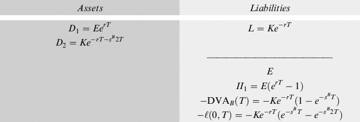
Equity is now incremented by interest II₁ earned on the first bank account, and it is decreased by debit value adjustment at time T, DVA_B(T), and by the value of the amount of losses that can be attributed to period [0, T], . It is very interesting to notice that:

so that the balance sheet above can be rewritten in a totally equivalent way as:

This choice of bookkeeping stresses the fact that, even in a multi-period setting, the value of the loss is still the DVA of the operation computed at contract inception, compounded at each period with the risk-free rate. The first choice above, on the other hand, allows for their attribution to each period by isolating the losses. This is also true of variable (possibly stochastic) spreads and interest rates.

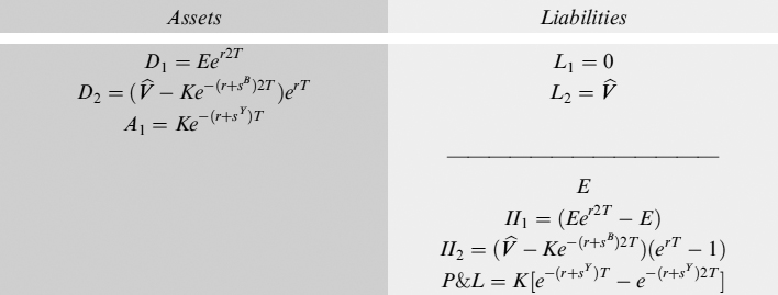
Time 2T

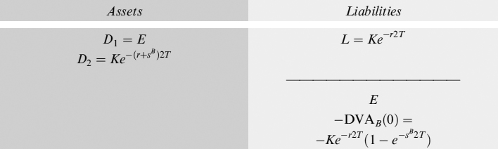
Let us see what happens at 2T, when the loan expires and the bank (i.e., the borrower) closes the business. In this case we have once again interest accrual at T, while DVA is nil and the losses that have to be updated must also include those referring to the second period:

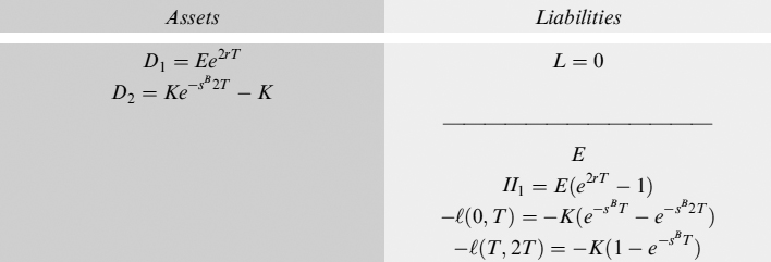
Once more it is quite easy to check that the assets and liabilities balance. It is also interesting to notice that:

which confirms what we have stated above, that total losses over the contract period are the future value of DVA computed at the start of the contract and that the funding spread (and the risk-free rate) can also evolve stochastically until maturity, since eventually only the initial level of the spread is what really counts. Evolution of the funding spread matters only in the attribution of portions of the total funding costs to a given period, something that is definitely important for performance measurement purposes, under the assumption that the funding cost component has to be assigned on a mark-to-market basis.

We also calculate in this case the profitability of the bank's activity during its life, considering the hurdle rate for the invested capital, thus getting:

so that the starting equity invested has been eroded by total funding costs.

Our analysis clearly shows that the question about whether to consider DVA or not in the balance sheet, since it apparently generates perverse effects, is actually ill posed. In reality, DVA is not a reduction of the current value of liabilities, but simply the present value of costs the counterparty has to pay to compensate other parties for the fact that it is not risk free. Given Axiom 10.2.1, the same amount is seen as a cost from the borrower's perspective, and as default risk compensation from the lender's perspective.

Viewed as the present value of cost, DVA is the reduction of the equity that can be determined from the start of the contract, although its monetary manifestation may occur only at maturity. As such, it can be included in the (marked-to-market) balance sheet in a consistent fashion as a reduction of equity, and no perverse effects manifest themselves if the creditworthiness of the borrower worsens, since the present value of costs increases and net equity is accordingly abated. From this perspective, DVA must be included in the balance sheet without any doubt, thus fulfilling the sound and prudent management principle.

10.4.3 DVA as a funding benefit

As mentioned above, several not totally satisfactory justifications for liability reduction as a result of DVA have been provided in recent works. Some authors⁹ present a list of arguments on how to manage and monetize DVA, along with related pros and cons. They also warn, however, about the very delicate nature of DVA inclusion in the balance sheet.

Some other authors¹⁰ argue that DVA should actually be viewed as a funding benefit, thus apparently fully justifying its insertion in the balance sheet as a reduction in the current value of liabilities. However, in our opinion, the argument is not justified.

Anyway, let us check if this argument somehow impairs our notion of DVA. Assume we are in a multi-period case, and we are at time T: at this moment the borrower asks for more funds from the lender, starting a new loan contract for an amount K₂ < K, to be paid back at time 2T, together with the other loan K. K₂ is deposited in a (risk-free) bank account D₃. The balance sheet at time T, with the updated DVA, now reads:

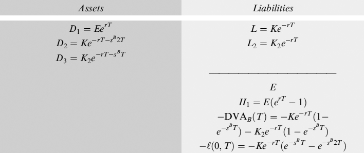
Those in favour of the “funding benefit” argument (implicitly) suggest that cash should not be deposited in a bank account (D₃ in our example), but should be used to buy back some debt, thus reducing the funding need. Nothing prevents implementation of this strategy, so that the balance sheet, after buying back a portion of the first loan, is:

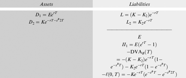
DVA_B(T) is reduced consistently with the reduction of the debt whose original amount was K. The balance sheet at the end of activities 2T is:

It is quite easy to check that total loss is simply:

or, the cost paid on the total amount borrowed K + K₂, considering buyback of debt K₂, which leaves total outstanding debt K equal to the staring amount. So, if we define funding benefit as reduction of the funding cost for a given amount of raised funds, we can easily see that, given the net total amount funded over the period (K in our case), there is no reduction in cost, which remains exactly the same as before.¹¹

Now, we do not want to discuss how sensible the strategy of issuing debt (i.e., borrowing money) and immediately buying back issued debt is, rather we want to stress the fact that if, for whatsoever reason, the borrower has money to reduce its outstanding debt, he is at the same time correspondingly cancelling part of the DVA shown in the balance sheet. In other words, the present value of the costs due to the funding spread can be reduced when the borrower has available free cash to buy back his own debt. If available cash is obtained by a new loan, no real funding benefit can be achieved; this is also true if the cash is originated by a derivative transaction (e.g., selling an option), as we will see below in more detail.

The “funding benefit” argument does not seem to truly justify consistent insertion of DVA on the balance sheet as a reduction in the value of liabilities, even if one looks at it as a funding benefit and not from the perspective of counterparty credit risk, which we already criticized above. Actually, even in the reasoning presented above we are not referring counterparty credit risk at all, we are simply referring to costs, provided that Axiom 10.2.1 holds. Nevertheless, we need to investigate the argument further and will do so later on.

It is worthy of note that our notion of DVA does not exclude the possibility that the borrower may enjoy a reduction in his liability value: if the interest rate rises, the present value of the loan decreases. Whether this profit can actually be realized depends on the composition of the assets of the borrower, since available free cash is needed to buy back the loan.

10.5 DVA FOR DERIVATIVE CONTRACTS

CVA and DVA are concepts devised for OTC derivative contracts as measures of counterparty credit risk. As such, they are improperly used for loan contracts, but ultimately their application offers a good conceptual framework to decide how to properly include the credit risk of the debtor too in the balance sheet, and to precisely disentangle the contribution to total P&L of the several cost and income components.

When dealing with OTC derivative contracts, the main difference is that the exposure that one or both counterparties have to the other party is stochastic over time. We will investigate how DVA can be entered on the balance sheet and how to interpret it in this case.

We analyse a very simple derivative contract: a forward contract on asset S. The main setup is the same as above: we assume that the bank (which is now no longer a borrower) B strikes a deal at 0 to buy at T one unit of the asset at price X. We also assume, to simplify things, but with no loss of generality, that the counterparty of the bank is risk free, so that we do not have to consider any CVA in the analysis. The bank can only default at the end of activities at T.

The value of contract H(0) can be derived according to standard techniques¹² as:

where E[] is the expectation operator and DVA_B(0) is (assuming independence between default probability, asset price and zero recovery on default):

In words, DVA is the discounted expected negative value of the contract at expiry, weighted by the probability of default of the bank. This is the loss that the counterparty may expect to suffer, given the default of the bank. The fair forward price is the level of X making nil the value of the contract at inception:

so that:

It is manifest that the bank can close a forward contract at conditions worse than those it can get if it were risk free. In fact, B buys at expiry the underlying asset at price X > X^rf, where X^rf = E[S_T] is the fair forward price if B cannot go bankrupt, and hence DVA_B(0) is zero.

Let us consider how to include a forward contract in the balance sheet (the equity is the same as in the case examined above). The value of the contract has to be computed by discounting the expected terminal value of the contract, plus expected losses due to counterparty risks (i.e., CVA, which is nil in our case by assumption) and other costs (DVA in the framework we have suggested). The value of the contract to B is:

which is negative and a (positive) liability (although it should be noted that the value may change sign at any time until maturity, and hence become an asset). The bank has to recognize a liability due to the mark to market immediately after closing the deal, and this is equal to the DVA of the contract, as just shown. On the other hand, it also has to consider DVA as the present value of costs due to the fact that it is not default risk free. So the balance sheet reads as:

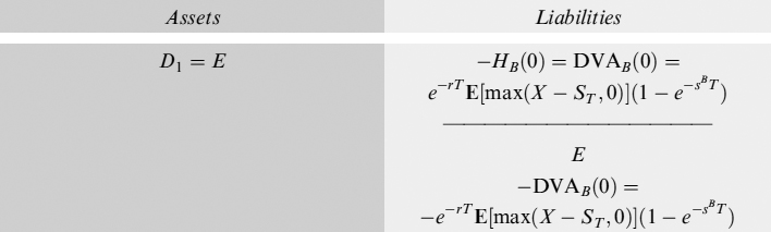
Assets and liabilities clearly balance and we are consistently considering the value of the contract and related extra costs borne by B. In this way, closing the deal generates no further P&L.

We now have to check what happens at time T. Assume that underlying asset price S_T is equal to the expected price at the contract's inception S_T = E[S_T]: the bank then suffers a loss calculated from the value of the forward contract as follows:

The balance sheet in T is then:

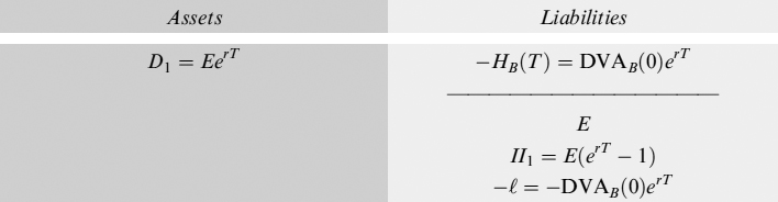
The loss has to be financed by the cash available in the bank account, where the original equity was deposited, so that the final form of the balance sheet in T is:

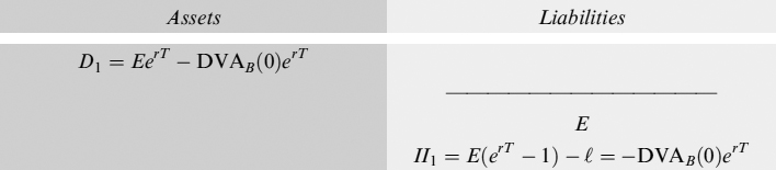
This confirms the fact that the DVA for a derivative contract is also the present value of a cost. Anyway, the definition can be slightly refined by moving one step forward. In fact, let us assume that the underlying asset's price at expiry T is some S_T ≠ E[S_T]: the value of the forward contract is then:

which may result in a profit or a loss, depending on the level S_T. Anyway, when this value is compared with the corresponding value of a forward contract whose fair price was determined by assuming that B is a risk-free counterparty, it is straightforward to see that:

So DVA is a cost that worsens losses, or abates profits, at expiry T with respect to the same contract dealt by a risk-free counterparty: this cost is once again due to the fact that the bank is not a risk-free economic agent. If we introduce a multi-period setting we will have the same conclusion as above:¹³ variability of the DVA allows allocating portions of total costs on different subperiods, but it is immaterial to determining total cost, which is still the DVA calculated at the start of the contract.

It is also worth analysing what happens with derivatives starting with a nonzero value at inception, such as options. Some authors¹⁴ recently provided a proof on how to replicate a derivative contract including CVA, DVA and funding. Their approach relies on the bank trading in the counterparty's bonds to replicate the CVA and its own bonds to replicate the DVA: the argument hinges on the funding benefit that can be received by buying back its own bonds. The existence of issued bonds to be bought back is assumed, otherwise a replica would not be possible: if we accept this assumption, DVA inclusion in the balance sheet, as a correction of the contract's value, would be fully justified because it can actually be replicated. Let us check if this is true.

At time 0, let bank B sell call option O expiring at T to a counterparty, struck at level X. The value of this contract is its risk-free value minus DVA, with no CVA since the bank has no exposure to the counterparty.¹⁵ The value can be written as (with the same assumptions made for the forward contract):

where the DVA_B(0) is:

We include this contract in the balance sheet, where there is also a debt. The value of the debt is equal to the value of the option and is deposited in a risk-free bank account D₂. The value of the option contract to the borrower is risk-free premium V(0) = O(0)+DVA_B(0) = O^rf(0), and DVA_B(0) is accounted for, according to our proposed notion, as a loss:

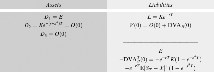
where is total DVA including the option's and the debt's. Now, according to those supporting DVA replication¹⁶ the replica generates enough cash to buy back the debt. In fact, in our example we have cash deposited in account D₃ equal to the premium received.¹⁷ This can be used to buy back outstanding debt, whose value is equal to the premium, as assumed above to make things as simple as possible. So the balance sheet now reads:

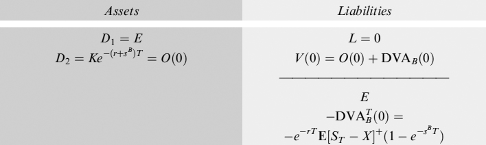
The debt is now nil and DVA has been updated. The funding benefit has to be verified at expiry of the option, when the option is worth O(T) and its DVA_B(T) = 0. The P&L generated by the option is −(O(T) − O(0)e^rT) giving:

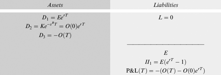
We do not appear to have suffered any loss deriving from DVA, but this is a false perception. Actually, if DVA is the extra cost the bank has to pay for not being risk free, then if we compare the final P&L with respect to the P&L of a risk-free bank we get:

So the P&L has a hidden cost that is not only equal to DVA_B(0)e^rT, but also to the compounded DVA on the outstanding debt before it was bought back. So, given the funds available to the bank over the period, which are equal to O(0), the losses incurred are in every case of DVA_B(0) explicitly or implicitly shown in the balance sheet. In the end, even the argument of buying back the bank's own bonds does not justify inclusion of DVA in the balance sheet to reduce liabilities, as expected after having criticized the “funding benefit” argument above.¹⁸

We would like to stress that we are not saying that the replication strategy is wrong because it is impossible to buy back issued bonds, or that the assumption of existing outstanding debt is weak (although no issued bonds being available is something that may actually happen). We believe we have only proved that, however you define it, abating liabilities using DVA is an accounting and financial mistake, apparently subtle but with huge practical impacts that are analysed in more depth later on in this chapter.

We are finally in a positon to propose the following definition, which encompasses all the cases we have analysed so far.

Definition 10.5.1. Debit value adjustment (DVA) is the compensation a counterparty has to pay, when closing a contract, to the other party to remunerate the default risk that the latter bears and that is specularly measured as credit value adjustment (CVA).

This compensation is the present value of the extra costs (given Axiom 10.2.1) that the counterparty has to pay with respect to a risk-free counterparty and as such it must be included in a marked-to-market balance sheet as a reduction of equity.

In a multi-period setting, the portion of the initial DVA attributed at each period may depend on the stochasticity of the probability of default of the counterparty, and of the underlying asset of the contract, but in any case the total cost over the entire duration of the contract is still the DVA calculated at the beginning of the contract.

10.6 EXTENSION TO POSITIVE RECOVERY AND LIQUIDITY RISK

In the analysis above we assumed that the loss given default of the exposure is full (i.e., L_GD = 100%), and that the liquidity spread is nil (γ = 0). In this section we release these two assumptions and we analyse which effects are produced after that.

Let us start with the case when L_GD < 100% and γ = 0. It is very well known that the spread, in a reduced-form setting to model credit risk when recovery is a fraction of the market value, is:

This can be seen as an approximation of the formula for loss given default on an exposure of amount K: L_GDK(1 − e^−πT) ≈ L_GDπTK ≈ K(1 − e^−sT), with s = πL_GD. When valuing the expected value received at expiry T, one gets:

thus confirming equation (10.9). Given market spread s and assuming loss given default L_GD, we can derive the probability of default trivially as: π = s/L_GD.

With this information at hand, it is quite straightforward to adapt the framework above to the case when L_GD < 100%. Actually, CVA (equal to DVA from the borrower's perspective in formula (10.2) can be written as CVA_B = DVA_B = L_GDBKE[1 − 1_TB>T] ≈ K(1 − e^−sBT). On the other hand, funding cost FC_L is computed with s^L, which is now equal to π^LL_GDL instead of simply π^L, but this change will not affect our subsequent analysis at all.

We now add a liquidity premium γ ≠ 0. When included in the lender's spread, we have that s^L = π^LL_GDL + γ^L, and this is the new spread to insert in quantity FC_L of equation (10.2), but no other effects are produced.

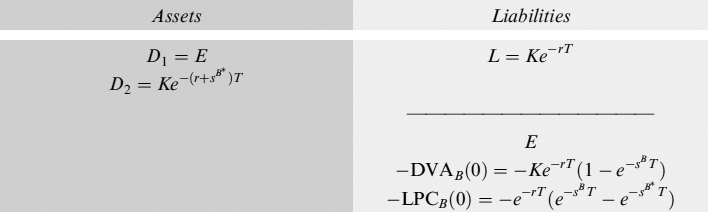
For the borrower's spread the treatment of the DVA deserves more attention.¹⁹ Let us define the spread including the liquidity premium as s^B* = π^BL_GDB + γ^B and the spread including just the credit component as S^B = π^BL_GDB. Now equation (10.3) has to be modified as follows:

and we have

where

is DVA, and

is the liquidity cost due to liquidity premium γ^B. Quantity LPC_B is an extra cost that is in all respects equal to DVA for the borrower and, hence, has to be included in the balance sheet as a reduction of net equity, similarly to DVA:

The analysis then can easily be extended to consider costs related to liquidity as well.

It is worth stressing here that the sum of DVA_B and liquidity costs LPC_B is just the total funding cost FC_B for the borrower. In fact, if the borrower takes money from economic agents who do not pay any funding spread, such as investors, then it is easy to see that (from the definition of P_B):

If the borrower also has to pay the funding spread charged by a lender who has to fund the activity, such as a bank, then one gets:

where IC_B is the intermediation cost that the borrower has to pay to the lender for not having direct access to the capital market, and it is defined as:

Although we left it unspecified, the funding cost of lender FC_L is actually the sum of his DVA_L (and intermediation costs IC_L in this case) and liquidity costs LPC_L.

We are now in a position to give a definition of the funding cost for loan and derivative contracts

Definition 10.6.1. The funding cost FC for a loan contract is the present value of extra costs, with respect to a risk-free operator, that a counterparty has to pay for the liquidity premium, for intermediation costs for not having direct access to the capital market, and to compensate the other party for the default risk that the latter bears.

The funding cost FC related to a derivative contract is the sum of funding costs that a counterparty has to pay on money it borrows to match negative cash flows. Given that the present (risk-free discounted) value of the sum of (expected) negative and positive cash flows is nil when the contract is fairly priced, borrowing of money is only needed when cumulated cash flows are negative during the life of the contract, before receiving counterbalancing flows. So, funding costs for a derivative contract depend on the cash flow schedule which determines whether they materialize or not.

From Definition 10.6.1 we can deduce that, assuming no liquidity premiums and intermediation costs, the funding cost and DVA are one and the same thing for a loan contract. For derivative contracts DVA is completely unrelated to funding costs, which can be seen as the sum of DVAs relating to loans needed to fund negative cumulated cash flows during the life of the contract. Evaluation of these costs has to be carried out on a case-by-case basis, depending on the type of contract and even on the position (long/short) that the counterparty is taking in it. We will examine these aspects in greater detail in Chapter 12.

10.7 DYNAMIC REPLICATION OF DVA

We now investigate more thoroughly the feasibility of dynamically replicating the DVA. If it is, then DVA is a quantity that can be fairly deducted from the liabilities of a financial institution. In this case, the argument of such works as [42], where a dynamic replication strategy is derived in great detail, could be accepted. If, on the contrary, it is not feasible, then DVA should be considered a cost and as such should be deducted from the equity of the financial institution. In this second case we confirm the results we derived above.

We will analyse the problem from a very wide perspective. We will show that dynamically replicating the DVA hides very subtle assumptions about the composition of the balance sheet of the financial institution. We will also point out the (negative) consequences for the financial institution if it organizes its derivative business so as to hedge and also replicate the DVA and we will demonstrate how the bank's franchise will be gradually eroded.

10.7.1 The gain process

We start from a very basic concept in option pricing theory. It seems that we are just repeating very well-known results, but we do so because we do not understand why these results are strangely forgotten when DVA is involved in the analysis.

Let X_t be the stochastic variable representing the price of an asset. The evolution of X_t is given by the following SDE (Ito process):²⁰

Define a trading strategy as an adapted process θ specifying at each state ω and time t the number θ_t(ω) of units of the asset held by an economic operator. The gain process generated by θ is the stochastic integral:

Basically, the gain process indicates the gains (which can be both positive and negative) generated by θ_t units held at each time t given variation dX_t of the asset.

Assume we have a constant quantity held between time T and T′. The gain process is simply . It is immediately apparent that the gain process is nil with probability 1 between the two times T and T′ if .

Assume now we short one unit of the asset between 0 and T and buy it back between T and T′, so that θ_t = −1 for t ∈ {0, T} and θ_t = 0 for t ∈ {T, T′}. The total gain process is:

The calculations are pretty simple and lead us to trivially state that when we do not hold any quantity of the asset for a given period we do not earn any gain.

The asset can be a stock, a commodity or a bond. When a financial institution (say, a bank) issues at time 0 a bond (X = B) to finance its business activity, this is the same as going short (i.e., sells without having previously bought) the same bond (θ₀ = − 1). Assume for simplicity, but with no loss of generality, that it is a zero-coupon bond. The bond is usually paid back at expiry T by the bank, which is in practice buying back the bond shorted (θ_T = 0), and the gain process typically entails a loss for the issuer (−1 × [B_T − B₀]) which is the amount of interest granted to the bondholder. The bond can be bought back even before expiry, at time u < T, thus producing a gain − 1 × [B_u − B₀] that could be positive or negative if we are in a stochastic interest rate and default probability economy. On the other hand, if we are in a deterministic interest rate and default probability economy, buying back issued bonds always implies a loss for the bank, although lower than that suffered at expiry (i.e., the bank pays less interest, since it keeps a short position in the bond for a shorter period). It is clear that, from time u until expiry T, the gain process is nil since θ_t = 0 for t ∈ {u, T}, unless the bank decides to issue the same bond once again.

10.7.2 Dynamic replication of a defaultable claim

Dynamic replication relies on getting the same payoff structure as a derivative contract via a trading strategy in primary securities (e.g., stocks and bonds). Assume we have a vector of N securities defined by the price process X = (X¹, …, X^N). We want to replicate dynamically a derivative claim whose terminal payoff at expiry T is V_T and whose initial price at time 0 is V₀.

The replication portfolio is set up at 0. We have to find a trading strategy θ such that it satisfies the following well-known conditions:²¹

1. Self-financing condition: No other investment is required to operate the strategy besides the initial one:

   

2. Replicating condition: At any time t the replicating portfolio's value equals the value of the contract and of the collateral account:

   

   for t ∈ [0, T].

We apply replication to a defaultable derivative contract whose corresponding default risk-free value is denoted by V: the deal is written between bank B and counterparty C. In building the replication portfolio we strictly follow [42], to which we refer for details. is the value of the contract seen from counterparty C's perspective and is also the value bank B has to replicate once it closes the deal, so as to hedge the exposure it has towards C.

Since we want to investigate whether CVA and DVA can be replicated, we exclude any collateralization and/or credit risk mitigation agreement, which would reduce or eliminate these two quantities. Moreover, we do not consider agreements related to credit-rating triggers, such as the rating-based termination events analysed in Mercurio et al. [91, second part of reference]: in case there are such agreements, the results we derive below will require further adjustment.

Let X¹ ≡ S be the underlying asset on which the contract's payoff is contingent, X² ≡ P be a risk-free zero-coupon bond, X³ ≡ P^B be a default-risky zero-coupon bond issued by bank B and finally X⁴ ≡ P^C a default-risky zero-coupon bond issued by counterparty C. The two risky bonds depend on the respective issuer defaulting, so that they can be used to hedge exposures the derivative contract implies to party defaults. Both bonds have zero recovery if the issuer defaults.

The dynamics for S are the same as in (10.11), whereas the dynamics for the bonds are:

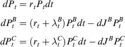
where r_t is the deterministic time-dependent instantaneous risk-free interest rate and λ^I is the yield spread of operator I ∈ {B, C}, which in equilibrium should also be the instantaneous default intensity.

We apply Ito's lemma to the value function , where J^B and J^C are two point processes that jump from 0 to 1 on default of, respectively, B and C with default intensity λ^B and λ^C. We get:

where we used the operator L^a· defined as:

and we set variation of the contingent claim value on default of one of the two parties as:

and

On the other hand, bank B wants to build a replicating portfolio comprising quantity Δ_t of underlying assets, of zero-coupon bonds issued by the bank itself, of zero-coupon bonds issued by counterparty C, and finally an amount of cash β_t, so that it satisfies the two conditions stated above:

and

Quantity β_t is defined as:

and its evolution depends on the assumptions made on how to finance the asset and the two bonds.²² We assume that the position in the underlying asset is financed by a repo transaction: if the repo rate is r^R and the asset grants continuous yield y, then for this part cash will evolve as:

The position in the counterparty's bonds can be financed at repo as well, and we assume there is no haircut and a repo rate equal to the risk-free rate r, so that evolution for this component of the cash is:

Finally, the position in the bank's bonds can be financed by the amount that the replication strategy implies as an investment at the start of the contract; any remaining sum of cash will be invested at the risk-free rate if positive, or financed at the risk-free rate plus the bank's funding spread S^B if negative, thus yielding the dynamic for this last part of the cash:

Collecting the results we eventually get:

By equating (10.18) with (10.15) we can derive the quantities of the different assets to include in the portfolio so that it perfectly replicates the derivative contract. It can be shown that they are:

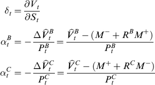
where we have defined M as the mark-to-market value of the contract upon default of one of the two parties and R^I, I ∈ {B, C}, as the recovery fraction of the contract paid by defaulting party I to the other party.

By rearranging terms, it can be shown that the final PDE, whose solution is the value of the derivative contract, is:

If we assume that the mark-to-market value on default of one of the parties is the defaultable value of the contract, then .²³ In this case the total value of the contract can be decomposed as (i.e., a risk-free component plus an adjustment due to credit events), which is the solution of the PDE:

where V is known and can be derived by standard techniques. Application of the Feynman–Kac theorem provides the solution to the adjustment term as:²⁴

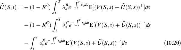
Formula (10.20) contains two elements related to counterparty credit risk: the right-hand side of the first line shows the CVA (from C's perspective) and is the correction to the risk-free fair value V needed to remunerate the risk C bears for B's default (recall that value V is seen from C's perspective); the second line is the DVA (again, from C's perspective) and is the correction needed to remunerate the specular risk that bears for C's default. Finally, the third line, shows the cost bank B has to bear when trying to replicate a long position in the contract, which is related to the funding spread it pays over the risk-free rate.

Since we are interested in studying the effectiveness of the replication strategy of U(S, t) from bank B's perspective, and more specifically its DVA, we will focus on the DVA from this perspective (i.e., the quantity in the first line of (10.20)); in mirror-image fashion, the DVA from counterparty C's perspective (second line in (10.20)) is in fact the CVA for the bank.

Let us take a closer look at the sign of the quantities the bank has to hold in the portfolio to replicate U(S, t) and hence to hedge its mirror-image position − U(S, t) against counterparty C.²⁵ The CVA (or DVA from the counterparty's perspective; second line in (10.20)) can quite easily be replicated by selling an amount of bonds issued by counterparty C equal to : this can be achieved in a simple way by a repo agreement with a third party, or even in more heterodox ways such as buying credit protection via a CDS (with all the related caveats). The funding component of U(S, t) (the third line) is also not very worrisome in terms of replicability: the bank has to issue new bonds to fundagainst any negative cash flow originated by setting up the replication portfolio. Provided there are no liquidity issues in the market, borrowing money from other operators should be a straightforward matter.

Replication of the DVA (i.e., the CVA from the counterparty's perspective; the first line in (10.20)) is trickier: it entails the bank going long a quantity of its own bonds equal to . Now, while going short its own bonds is relatively straightforward for the bank, since in the end it amounts to borrowing more money from the market, going long its own bond is not possible, although this is often overlooked in the literature. Actually, Burgard and Kjaer [42] also suggest an apparently simple way for the bank to go long its own bonds by buying back bonds issued in the past. Although in theory one cannot exclude the possibility that a bank has never issued bonds in the past, in practice the strategy is admittedly not very difficult to implement: in fact, banks regularly issue debt and there are many bonds in the market to buy back. So, is buyback a strategy to go long its own bonds for the bank? The answer is definitely not, and the reason is not because we object that is quite hard to find an issued bond in the market that exactly matches the features of bond P^B needed for the replication strategy. We claim there is a more fundamental reason the buyback strategy is not effective.

In fact, there is a difference between buying a security and being long it. We stressed that in Section 10.7.1, when we somewhat redundantly showed that buying back a short position clearly makes the net position nil for the dynamic replicator: if the replica prescribes a long position in a given security, the replicator should keep on buying until she is net long the security. But when a bank buys back its own bonds, it is simply reducing its short position or it is making it at most equal to zero, by not going long its own bonds (i.e., adding a positive amount in its portfolio). The gain process for the bonds bought back stops (since the quantity of the “bond” asset θ = 0, using the notation in Section 10.7.1); from the time of the buyback on, the gain process simply sticks to the amount of profits or losses generated since the issuance of the bond and no other variation occurs. So, replication of the DVA (from the bank's perspective) simply does not happen since there is no actual contribution from the gain process of the bank's bonds. Despite the robustness of this statement, it hinges on the belief that it is not possible for the bank to go long its own bonds in any fashion. However, our statement may be subject to possible critiques that we both devise and rebut in the next section.

10.7.3 Objections to the statement “no long position in a bank's own bonds is possible”

As a first attack on the statement “No long position in a bank's own bonds is possible”, we may object that despite it being true that the bank never really goes long its own bonds, if we consider the replication strategy as a closed system, then the bank is actually long the bond such that replication is effective. This objection is based on an “abstract concept of an abstract concept”, as proposed by philosopher Emanuele Severino.²⁶ The long position of the bank in its bonds within the closed system “dynamic replication of its DVA” without considering the total net position of the bank within its balance sheet (i.e., the total of its assets and liabilities to which the “dynamic replication of its DVA” subsystem also belongs) is an abstract concept: being long in the subsystem means that a short position is opened somewhere else in the total “balance sheet” system, so as to preserve the zero position in the bank's own bonds at an aggregated level. So in the end the bank is long in the “dynamic replication of its DVA” subsystem and short somewhere else in the overall “balance sheet” system. Moreover, assuming the long position in bonds actually exists and produces effects is an abstract concept as well, since at an aggregated level the effects just offset each other.

In the end the bank cannot attain an effective long position in its own bonds, although it is possible at the subsystem level to assume this position. Nevertheless, it still has to be counterbalanced at the system level by an opposite position. This means that if replication of the DVA is formally attained in the “dynamic replication of its DVA” subsystem, in practice replication is simply paid by abating some assets or increasing some liabilities in the “balance sheet” system, so that the net total result is that the replication strategy ends up as a loss (in other words, as a cost) for the bank. This is simply due to the strength of logic consequences and with this in mind we will be better equipped to face another possible critique as well.²⁷

The second, and somehow subtler, critique we may raise to the impossibility of having a long position in bonds is based on the “funding benefit” argument; that is: if the bank has money to buy back its own bonds issued in the past, then it gets a benefit in terms of the smaller funding costs it pays on outstanding debt. So, despite the critique implicitly accepting the statement that it is not possible for the bank to go long its bonds, it introduces the gains, or benefits, the bank obtains with a smaller outstanding debt. Funding benefits are also mentioned in [42] and [94], although in vague terms. To be completely honest, this argument does appear to hold water, but we have to investigate it further to ascertain its validity.

Granted, for the sake of argument, that the funding benefit really exists,²⁸ it is not clear how it is related to replication of the bank's DVA and how its variations actually track variations in DVA.

10.7.4 DVA replication by the funding benefit

Keeping our discussion in the previous section in mind, what is undeniable is if a bank has some cash and can buy back all or some of the bonds issued in the past, then it reduces the amount of debt. This is not precisely a funding benefit, which in our opinion should be defined as a saving of funding costs given a certain amount of debt, but can be loosely thought of as a benefit since the bank has to pay less interest, taken as an absolute value. So we loosely define funding benefit as deduction of the amount of paid interest that can be obtained by reducing total outstanding debt after buyback.

Since the replication strategy is formally self-financing, when it prescribes buying back a bank's own bonds, it is also generating the amount of cash needed to perform this. So we can be pretty sure that, as far as the DVA component is concerned, the bank has cash to buy back a quantity of its own bonds thus reducing its total outstanding debt. To investigate whether this amount of debt “missing” from the original total amount really contributes to replicating the DVA we need to to look at the entire bank's balance sheet and how assets and liabilities are originated.

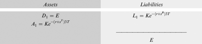
Let us commence with a very basic situation: when the bank starts its activities at time 0, with an amount of capital E, deposited in an account D₁ = E. We observe the bank's activity at discrete time intervals of length T. At 0 the bank also issues an amount K of zero-coupon bonds P^B with unit face value and expiring at 3T. Adopting the same notation introduced above, the amount of cash raised by the bank is Ke^−(r+SB)3T (recall that S^B is the bank's funding spread); this cash is used to buy K zero-coupon bonds P^Y, issued by a third party Y, with unit face value and expiring at 3T. The third party has a funding spread S^Y such that the present value of the bond is Ke^−(r+SY)3T; if both bonds have the same funding spread, S^B = S^Y, then the money raised by the bank is enough to buy the bond from issuer Y.

For the moment we assume that the funding spread is due to some unspecified factors and make no attempt to link it to default risk, which in reality should be the first cause of its existence. We will very soon consider default risk explicitly in the following analysis, but for now we simply disregard it. Continuing with our assumption, we can then affirm that the bank is operating a very simple replication strategy for asset A₁, with the opposite sign used to hedge it, via issuance of its own bonds.

The marked-to–market balance sheet of the bank at time 0 looks like:²⁹

Let us now assume one period T elapses and the bank closes a derivative contract. To make things more explicit and to avoid unnecessary complications (but in any case with no loss of generality), we suppose that bank B sells to counterparty C an option on some underlying S whose value to the latter is (this choice will allow us to exclude from the analysis the CVA for the bank, which is zero for short options); clearly, the option is worth the same to the bank but with the opposite sign. Since it has a negative value to bank B, the option is a liability; on the other hand, the premium paid by C increases the cash available to B and is deposited in deposits D₂. The balance sheet will then be:

Assets and liabilities accrue interest and a net profit (Ee^rT − E) is earned between 0 and T. The bank immediately commences its dynamic replication strategy as well: for simplicity's sake we only focus on the DVA part (from the bank's perspective) of the quantity U(S, t) in (10.20) (i.e., the CVA from the counterparty's perspective), without considering the Δ-hedge with the underlying asset. We assume that quantity α^B of the bank's bond to buy back is exactly equal to K, or the amount of the bond outstanding issued at time 0. Obviously, to buy back the bond, the amount of available cash in D₂ is abated correspondingly so that the balance sheet reads as:

We now get to the heart of the matter: no bond appears amongst the bank's liabilities, which seem to have declined. In reality, they have not declined, they have increased since the bond has been replaced by a short position in the option that is worth (negatively) even more. In any case, the bond issued to counterbalance asset A₁ no longer exists, and this is a fact: much as if the bank has a long position in the asset that does not need to be financed by cash, whose availability to the bank increased as is manifest by the amount in deposit D₂ that did not exist before. This can be termed “funding benefit”, as suggested above; apparently, this makes it possible to have assets in the balance sheet without explicitly paying (or by paying fewer) funding costs.

We have already shown this saving is but an illusion. Anyway, we would like to check here whether this apparent saving is effective in the replication strategy. It turns out it could actually be effective if a certain set of circumstances are true. We have already stressed that when the bank buys back its own bonds, it is not really going long, but is simply making its former position nil, considering things at the balance sheet level. The gain process that is needed in the replication strategy is only abstractly produced (just in case it is so at a lower subsystem level, such as a trading desk), but in practice it stops at buyback (although the gain obtained up to this instant is immaterial to the replication strategy of the DVA for the bank) and stays constant until a new short position is opened by issuing the bond once again.

On the other hand, we can now argue that asset A₁ is no longer hedged (i.e., replicated with the opposite sign) since the issued bond has been bought back. Furthermore, we can argue that another gain process actually starts as a result of this uncovered position. Indeed, after one more period elapses, the balance sheet reads as:

The amount of capital deposited in D₁ accrues interest II₁, so that related profits increase; interest II₂ that has accrued on deposits D₂ generates other profits . We further assume that the value of the option stays constant under a certain set of circumstances, so that it does not contribute to the period's P&L.³⁰

The balance sheet shows we are left with a profit equal to K[e^−(r+sY)T − e^−(r+sY)2T] which would not be generated if the bond issued by the bank had not been bought back. In fact, the issued bond would generate a perfectly counterbalancing loss K[e^−(r+sB)T − e^−(r+sB)2T] (since S^B = S^Y) and the total effect on the balance sheet would be zero.

On the other hand, and for the same reason of equal funding spreads, the profit appearing in this case is the same as the profit that the bank would earn if it had a “true” long position in its own bonds.³¹ If the replication strategy indicates a quantity , then in equation (10.18) (recalling we are working in a discrete time setting)

so the gain process is in reality working (although it is generated by an asset different than the bank's bond) and the replication strategy for the DVA (from the bank's perspective) is actually operating as expected. So, is the “funding benefit” argument correct? Should we then admit that the replication strategy suggested in [42] is right and that we were wrong above when we negated its effectiveness? As we hinted above, things are subtler than they may appear. Let us analyse the hidden assumptions under which the replication strategy is working.

First, we stated earlier that the profit earned after the bank's bonds were bought back is equal to the profit that the bank would have earned had it been able to actually buy its own bonds – this was easily proved in the example above. We assumed a constant spread, though, for both bank B and issuer Y : this is the reason we can be sure that the profit generated by bond P^Y is exactly equal to that generated by bond P^B. We can relax the assumption of a constant spread by introducing for both issuers a more realistic time-dependent spread , I ∈ {B, Y}. However, in this case we must make sure that, if the two spreads are commanded by a deterministic function of time, then they are commanded by the same function; alternatively, if funding spreads are stochastic processes, they have to follow the same dynamics and the same paths: starting from the same value, they evolve in the future precisely in the same way.

Second, we now have to explicitly consider the possibility of default by the bank and issuer Y: actually, the spread simply indicates that this probability is not zero. In an environment where there is no recovery upon default and no liquidity premium or intermediation costs, it is well known that S^I = λ^I, where λ^I is (as above) the instantaneous default intensity for issuer I. Assume now that the condition for the identity of time functions for deterministic spreads, or of the perfect correlation of stochastic spreads, is fulfilled. Then, equality is guaranteed only if either bank B's or issuer Y's default occurs in the interval of time T. Either default, though, affects the effectiveness of the replication strategy in different ways.

In fact, if the bank goes bankrupt before issuer Y, then the replication strategy would still work, although it will be very likely stopped, as the rest of the bank's activity and the default procedure would kick in to start to pay creditors, if possible. So, in this case right up to the time of default of the bank, the replication strategy works and afterwards it no longer needs to work so that issuer Y may default at any time without material consequences (for the limited scope of the replication, of course).

If issuer Y's default occurs first, then the replication strategy fails completely and replication is not attained. Thus, when default is considered, another condition we must add to those above is that issuer Y's default has to occur after bank B's default. We can slightly relax this assumption and accept that they may happen together: in this case replication is attained up to the last instant needed by the bank and hence has no negative consequences on strategy.

Armed with these results, we can recapitulate the conditions under which the “funding benefit” argument is valid and DVA (from the bank's perspective) is effectively replicated:

1. The spread over the risk-free rate (the funding rate) of the asset and of the bank's bond must start at the same value at inception of the replication strategy and they must be driven by the same deterministic function of time or they must be commanded by two identical, perfectly matching stochastic processes.
2. The times of the default of bank B and issuer Y must be perfectly correlated so that when either defaults, so does the other.

These conditions are trivially fulfilled when issuer Y coincides with bank B, but we know that in this case it is impossible for the bank to go long its own bonds. In other cases conditions can only be imperfectly, or not at all, fulfilled and the replication strategy will not be effective.

Moreover, it should be stressed that the analysis presented refers to a very simplified situation, where the “bond” asset A₁ can be clearly isolated from other assets and its variations can be compared with those of the bank's DVA. In reality, the composition of assets is pretty complicated, such that it would be an extremely hard task identifying which bond has to be considered to measure the funding benefit for a given derivative contract.

10.7.5 DVA replication and bank's franchise

In bank management books, “franchise” is defined as the value the bank is able to create from its branch network, its systems and people and from its customer base and brand. According to the widely supported “special information hypothesis” proposed in [19], banks play a unique role in financial markets because they have private information about costumers unavailable to other, non-bank lenders (see also [22]). A different, not necessarily alternative, view is that the franchise value of banks originates in their provision of liquidity and payment services to their customers. That is, banks are special institutions not because of their privileged information with respect to other lenders but because they can grant funds more easily than other economic operators. The hypothesis is presented and tested in [113].

However originated, banks create a franchise if they are able to buy assets yielding more than required by the risks they embed or if they are able to issue liabilities at a level lower than their fair value. This can be done, for instance, by trading in assets mispriced in the market: the franchise value of the bank is increased by the skills³² of the traders and asset managers in this case. Although it is quite rare, sometimes in fact financial markets work efficiently, as happens when liquid assets are traded. For example, let us go back to the case we have analysed in the previous section: if we assume that the spread over the risk-free rate yielded by bond P^Y is due only to default risk and that recovery is zero, so that S^Y = λ^Y (the notation is the same as above), then if the market prices the risks correctly, the expected return over a small period dt is:

In this case the bank franchise does not really increase, even if the spread over the risk-free rate is positive. On the contrary, the bank is actually losing money on an expectation basis, since the funding spread on bank's liabilities has to be paid anyway, so that they instantaneously accrue interest at rate with certainty³³ and asset A₁ = P^Y yields just an expected risk-free rate r_t.

Another way to create the franchise is to charge a margin over the fair rate that remunerates risks and costs and provides for a profit, when the bank lends money to clients that have weaker bargaining power: especially retail ones that do not have easy access to capital markets. Going back to the case above, let us assume that bond P^Y is issued by a very particular obligor who is default risk free and does not have access to the capital market but can borrow money from bank B. In this case the bank may apply spread m over the risk-free rate which is simply a margin and not remuneration for the default risk. This means that expected return on asset A₁ = P^Y is r + m on an expectation basis. So, if m > S^B then the bank increases its franchise since it is able to generate profits in the future on a sound basis covering its funding costs. This is also true of a bank lending money to defaultable obligors if it is able to charge a spread S^Y = λ^Y + S^B + m′ that remunerates costs and risks (i.e., the bank's funding spread S^B and default risk λ^Y) and includes a positive margin m′.

When we considered the two conditions under which DVA (from the bank's perspective) can be effectively replicated, we mentioned that the default times of the bank and of obligor Y must be perfectly correlated. This condition is tantamount, from the bank's perspective, to assuming the possibility to buy an asset that is default risk free and yet yields more than the risk-free rate. In fact, when bank B does not default, neither does the obligor, hence when pricing the asset issued by Y and evaluating it against the costs and risks borne by the bank, the obligor's default does not need to be considered.³⁴

Under these conditions, if spread S^Y > S^B then the bank actually creates a franchise, notwithstanding the asset being defaultable. If S^Y = S^B then the bank just covers its funding costs without any profit margin. This is a very hypothetic and hardly realistic situation, but should it happen then the bank's power to apply this rate over the risk-free rate (which could also produce a franchise) is used to replicate DVA, thus confirming what we said above when we affirmed that replication of the DVA would end up, keeping the entire balance sheet in mind, as a cost that has to be covered by a margin above the risk-free rate on some other contracts.

Since the funding spread process of obligor Y and bank B, jointly with perfect correlation between the times of default of both, are conditions very unlikely matched in reality, the obligor's bankruptcy has to be considered in the evaluation process and spread S^Y is the remuneration for Y's default risk. So this spread cannot be used for replication of DVA.

On the other hand, if the bank is able to apply a margin over the rate needed to remunerate default risk, so as to compensate funding costs S^B, this margin can be effective in replicating the DVA, although the bank should be able to update it frequently, so as to track variations of its own funding spread. In other words, assets cannot be fixed rate bonds and spreads have to be reviewed not only to reflect the obligor's default risk but also that of the bank.

Moreover, the bank is here using its ability to finance some investments to cover losses represented by DVA. So DVA is formally hedged, but the cost has been indirectly charged to other business areas and eventually, considering the total level of funding available, the bank will always bear the same total funding cost.

In the end, should the bank receive some cash on closing a derivative contract, this can be used to buy back a quantity of the bank's own bonds. In this case the balance sheet shrinks, because an asset (the cash received) is used to abate liabilities (the bank's bonds): given the reduced amount of liabilities, there is a smaller cost to pay, and this will be equal to the DVA of the derivative contract (under the stated conditions). Were the bank able to buy assets yielding more than the risk-free rate on a risk-adjusted basis, with bonds issued before closing the derivative contract, and this extra yield was enough to cover funding costs over the risk-free rate of the bank's bonds, then it would be enough to cover the cost of the DVA too. There is nothing special nor a funding benefit here, simply reduced liabilities (balancing reduced assets) produce smaller funding to compensate for increased DVA costs.

The problem of considering rather naively the DVA as a funding benefit stands out more clearly when derivative contracts do not produce positive cash flows, as when the bank deals a forward or a swap contract, for example. In these kinds of contracts, with both parties starting at the zero value, DVA can either be paid immediately to the counterparty, and there is no way to treat it differently than a cost, or it can be embedded in the value of the contract by modifying the fair forward or swap price so that it is worse than the risk-free equivalent for the bank.³⁵ In this second case the bank could include the value of the contract in the balance sheet without separating the DVA component and treating it as a cost. However, according to the funding benefit argument, it should be considered replicable by a buyback of its own bonds as explained.

Table 10.1. Hedging of a short forward contract by a sell-and-buyback repo contract: bank position in the asset and cash of the bank at the start of the contract and at expiry

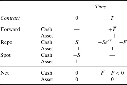
The impossibility of buying back bonds and then considering the DVA as a funding benefit is easily checked in this case, and we will show why: assume the bank sold asset S forward at future time T to a risk-free counterparty and that the fair risk-free forward price is F = Se^rT. Only the default risk of the bank has to be included in the valuation, so that the new forward price making the value of the contract nil at inception, which also includes the DVA, will be some .

In Table 10.1 we show how to hedge the forward contract and related positions in the underlying asset and in cash at the start and at expiry. Replication is attained with a strategy whereby the bank sells and buys back asset S by a repo transaction also expiring at T (we work under the assumption made above that the repo rate clashes with the risk-free rate). To deliver the underlying to the repo counterparty, the bank buys the asset on the spot market using the cash it receives from the repo sell leg. Then, at contract expiry the bank has to buy the underlying back from the repo counterparty: it will pay Se^rT = F against receiving one unit of the underlying, which will be delivered to the forward counterparty receiving an amount of cash equal to the forward price . The net result is that the bank loses an amount of money that exactly equals the DVA.³⁶

A bank strictly following the dynamic strategy indicated in [42] should also buy back a quantity of its own bonds, but since in a forward contract no cash is received at inception by the bank, the purchase can only be financed by resorting to a loan in the market, hence generating the ineffectual situation of replacing bank debt with equivalent bank debt, which produces no result at all.

Let us clarify matters by considering the DVA of the derivative contracts and of the issued bonds (for which DVA is exactly the funding cost) as costs reducing equity. If positive cash flows are received for whatever reason by the bank, then it can shrink the balance sheet by buying back outstanding debt, thus paying less interest on remaining liabilities. In this case, assets generating an extra yield covering the funding costs of bonds can be used to cover the DVA of derivative contracts, once they are bought back. If no positive cash flow occurs from derivative transactions, the balance sheet cannot be shrunk and both the DVA and the funding costs of the outstanding debt are costs to be paid in the future.

In conclusion, if we disregard the need, hardly met in practice, to update the spread for assets continuously and keep in mind that positive cash flows are not always received at inception, a bank that does not recognize the DVA as a cost when booking its derivative contracts, based on the false idea that it can be replicated, is implicitly using the margins that it is able (if it is ever able to do so) to charge on other products (typically, the banking book) to cover costs generated by derivatives desks (trading book). Simple buyback of its own bonds is not enough to justify the “funding benefit” argument if it is unsure as to which of the assets of other contracts is covering funding costs.

So, if a financial institution comprises only an investment bank arm trading in the financial markets, the derivatives desk would rely on the profits of other desks to cover DVA, so that the bank is destroying the franchise (in the event one is created).

If the institution also operates as a retail bank, the derivatives desk would rely on the ability of desks dealing contracts in the banking book to include funding costs as margins above the risk-free rate plus credit spreads in the pricing. Moreover, if the bank's spread is volatile, these margins should be reviewed frequently to align them with the current funding spread paid by the bank. All this hardly happens in reality so it is more likely that even in this case the bank would end up either by destroying value or by just covering total funding costs.

If the bank allows traders to implement replication strategies for DVA but fails to recognise this quantity as a cost, there are two immediate negative consequences.

First, when traders implement replication strategies, the bank uses margins generated in profitable businesses to cover the losses caused by the derivatives business losing money. In some cases this loss can be compensated by shrinking the balance sheet with cash flows received. So, at best the bank's franchise is not increasing; at worst it is actually being destroyed. This could be a very long and unclear process, especially when long-dated contracts are involved (e.g., a swap book), but the “bleeding” will be inexorable.

Second, traders (and possibly salespeople) think they can hedge the DVA and do not consider it as a cost, so no attempt is made to transfer it to other clients when dealing with them. If the bank is unable to avoid paying DVA on some trades or to charge the DVA of other deals that it has to pay on these trades, then the derivatives business is a lossmaker, so it is best to close it. This is equivalent to the bank lending money when it is not able to transfer its funding spreads to clients: sooner or later, the bank ends up losing money.

10.8 RECAPITULATION OF RESULTS

In the following table we recapitulate the main quantities studied above, their nature and the relationships existing amongst them.

Quantity	Nature
CVA = −DVA	Compensation for the counterparty risk borne by a party, given the exposure, the probability of default and loss given default.
DVA	Cost paid by a party that worsens the contract's conditions for a risk-free counterparty, given the exposure, the probability of default and loss given default.
IC	Cost paid by a party for not having direct access to the capital market.
LPC	Cost paid by a party for the premium required in the market to provide liquidity.
FC = DVA + LPC + IC	Cost paid by a party over the risk-free rate to raise funds. Some components may be nil.

10.9 ACCOUNTING STANDARD AND DVA

International accounting standards (IAS and FAS) agree on the inclusion of DVA in the fair value of the liabilities of a bank.³⁷ In other words, revaluation of liabilities taking into account the credit risk of the issuer (or of the counterparty with negative NPV in a derivative contract) is possible.

IASC [51], the board setting IAS accounting standards, tries to justify the inclusion of DVA as a liability reduction by saying:

This is the basis for conclusion (BC89) of the IAS 39 document: needless to say we consider the entire assertion to be weak. The first part astoundingly cites the “going concern basis” as justifying (also) a reduction of liabilities due to the credit spread of the issuer: we think we have demonstrated at length why DVA inclusion should be a reduction of net equity, which also entails a reduction in the value of equity when the credit standing worsens.

Moreover, point (a) is simply false as far as credit spreads are concerned,³⁸ except in the part referring to “repurchasing liabilities”, but in this case it is unlikely to have a widening of credit spreads (and hence a reduction of the value in liabilities) and to be cash-rich enough to buy back debt. Realizing revaluation profits “by using derivatives” means the bank selling CDS protection on its own debt, which is clearly not possible. Renegotiating debt means that that the bank is trying to update the interest it is paying on its debt, so as to get the new value of liabilities more in line with the notional value: from a financial perspective this new situation is exactly the same as the initial one.

Point (b) is a truism that does not need comment. Point (c) is probably the most sensible statement, at least it attempts to find a practical reason. Point (d) is again a truism. The last statement is frankly not even worth a comment, given its complete lack of rational sense (better, lack of comprehension of financial contract valuation).

According to [27], the board setting FASB standards:

Revaluation of liabilities including the entity's credit spread is then supported with claims such as:

Even in this case, although there is tentative justification on a microeconomic basis, the very slippery ground it stands on is patently indicated by the wording “but that increase probably is offset by losses that may have occasioned the decline in credit standing”. Beyond that, it is rather irrational to consider the value of liabilities from the creditors' perspective within the balance sheet, which represents the value of the company from the shareholders' perspective. To the debtor, the value of the liability is just the present value (discounted at the risk-free rate) of the notional amount (thus strictly adhering to the going concern principle). The comment “change in the position of borrowers necessarily alters the position of shareholders”³⁹ is true, but the balance sheet should report just the latter position and not mix both together. What is more, the correct representation of the bank's value to the shareholders is given if DVA is considered as a cost (loss) abating net equity.

DVA should be considered a cost to derivatives portfolios and as such should be deducted from equity.

In conclusion, we believe current accounting standards are not firmly grounded and they allow the accounting conduct of banks to produce very misleading information for those investors relying on balance sheet data. Hopefully, what we have shown above will contribute to better understanding of how to properly mark-to-market liabilities and how to represent costs related to the credit standing of the debtor (which are simply costs – not gains, as they appear according to existing accounting standards and practices). This is in accordance with the Basel Committee on Banking Supervision,⁴⁰ which not only explicitly forbids considering variations in DVA as P&L, but also makes clear that the DVA of derivative contracts at inception is a cost to be deducted from bank equity.

10.10 DISTINCTION BETWEEN PRICE AND VALUE

The difference between “price” and “value” has been investigated in economic theory, but economists (whether classical, neoclassical, or Marxist) typically reserve these terms for commodities. When a financial contract is not executed by simply (almost) immediately delivering an asset (in which case it can be assimilated to purchase/sale of a commodity) but, on the contrary, implies a given performance by possibly both parties for an extended duration, then price and value should be defined in a more refined way.

We define the “price” (from either party's perspective) of a derivative contract as the terms that both parties agree upon when closing the deal. These take into account the present value of expected profits and losses, while considering all the costs and losses due to counterparty credit risk, funding and liquidity premiums, for both parties. When both parties have even bargaining power, they have to acknowledge all the risks and costs the other party bears, so that the final price includes total (net) risks and costs borne by both parties.

On the other hand, we define the “production costs” (to one of the parties) of a derivative contract as the present value of the costs paid to attain the intermediate and final payoff until expiry, while considering the costs and losses due to counterparty credit risk, funding and liquidity premiums, related to that specific party. Production costs, assuming no other margin is charged, are how much the contract is worth to the party or, in other words, they are the “value” of the contract.

The price of a contract is an objective quantity, given by the level at which the two parties agree to trade the contract; the value of the contract is a subjective measure and is given by how much a contract is worth to one party. For either party the value of a contract should exactly equal the price – had it enough bargaining power – to completely transfer production costs (excluding other extra profit margins) to the counterparty, without recognizing during setting of the contract's terms the costs and risks borne by the other party. When the bargaining process involves counterparties with even bargaining power, then the value of the contract to each of them will be lower than the price as they are both yielding a share of the value to cover each other's risks and costs. The price and the value of a contract are also the same when both parties operate in a perfect and frictionless market, where there are no transaction costs and counterparty risks. In fact, in this case they will agree a production cost for the contract that is the same for both.

We have shown that DVA cannot be replicated using a dynamic strategy nor can it under very unrealistic assumptions justify the “funding benefit” argument. This does not mean that we do not have to consider bilateral counterparty risk when pricing a derivative contract. Neglecting transaction costs, which in practice further add to the final price of the contract, the bargaining process results in each party trying to include the relevant risks it bears in the price, so each party considers adjustments due to counterparty credit risk or CVA. This quantity can be replicated without any theoretical and practical hindering, since it is possible to trade short bonds issued by the other party. From the other's party perspective, the CVA is the DVA and since it cannot be replicated with a suitable dynamic strategy, it has to be considered a cost in the dealing price.

When the bank wants to compute the value of the contract, it has to consider itself a risk-free operator. The same is true for the counterparty. This does not mean that funding costs are not considered in the evaluation process, simply one's own default has to be excluded: this leads to cancelling DVA in the bilateral counterparty credit risk component from the traded price to determine the value to the party.

Let CVA^B be credit value adjustment due to the default risk of bank B, which equals DVA^B or DVA seen from the bank's perspective; analogously, let CVA^C be CVA due to the default risk of counterparty C, equal to DVA^C or DVA seen from the counterparty's perspective. Since each party considers itself default risk-free in the evaluation process, the value of the contract to C is:

On the other hand, the value of the contract to B is:

Let us consider the absolute value of the price of the contract and take the absolute values of the contract to each party. Both parties may acknowledge that the other party bears counterparty risk related to its default, even if when determining the value of the contract they exclude their own default risk. In practice, each party knows that it may be forced to yield something with respect to the value of the contract.

In other words, each party will trade at a price that includes a fraction (possibly all) of the CVA charged by the counterparty or, put another way, a price including a fraction of a quantity that cannot be replicated given by its DVA. Let 0 ≤ γ^B ≤ 1 be the fraction of CVA^B ≡ DVA^B acknowledged to the bank by the counterparty, and γ^C the fraction of CVA^C ≡ DVA^C acknowledged to the counterparty by the bank. The trading price p will then be:

where

When both parties yield 100% of their respective DVA to the other party (i.e., both parties can fully charge CVA and fully accept the other party's CVA), then we have traded price p equal to the price including full bilateral counterparty risk and the pricing formula would be the same as in [32]. The pricing formula would also be the same as the one derived in [42] and shown above, if the funding costs related to implementation of the replication stretegy (third line in equation (10.20)) are ignored. This price can be defined as the fair dealing price.

Funding costs are specific to each party and come about from the same default risk as the DVA. If we also consider funding costs, then the value to each counterparty would be even farther away from the fair price at which they can deal in the market. Denoting by FC^B the present value of funding costs paid by bank B in replicating the contract and, analogously, by FC^C the present value of funding costs paid by counterparty C, we can generalize the bounds within which the price of the contract deals:

and the dealing price of the contract p is now:

ζ^C and ζ^B are the fraction of the present value of funding costs borne by counterparty C and bank B acknowledged by, respectively, bank B and counterparty C.

To conclude, when default risk is considered, even in the absence of transaction costs, a unique value fair to both counterparties cannot be determined. The fair dealing price, if attained during the bargaining process, would in any case be at a level different from the values to both parties. All adjustments relating to counterparty risk can be replicated by both parties, but this does not mean that any adjustment can be replicated by any party: in fact, the DVA of each party can be replicated only by the other party, for which it is the CVA.

The ultimate conclusion is that derivatives trading, amongst professionals with equal bargaining power and without credit mitigation mechanisms, is a lossmaker for banks unless they also trade with weaker parties to whom they can transfer DVA-related costs (and funding costs).