
8.1 INTRODUCTION
In this chapter1 we present some models for market risk factors: all market variables, such as interest rates, credit spreads, FX rates, stock prices and commodity prices, are affecting the payoff of most of the contracts a bank has on its balance sheet. Effective and parsimonious models are required to allow simulation of the cash flows of contracts linked to the different market variables, which become risk factors in themselves.
We first introduce models that can be used to model the evolution of FX rates and equities, then we dwell on interest rate models and default models, which are the basis for the modelling of credit spreads. We do not focus on all market variables (e.g., we do not analyse inflation modelling), but hopefully we will cover the vast majority of the market risk factors that affect the cash flows of contracts.
The second part of the chapter, from Section 8.5 on, is devoted to application of the models to liquidity risk management.
8.2 STOCK PRICES AND FX RATES
A standard way to model the evolution of stock prices and FX rates is to assume that they are commanded by a geometric Brownian motion. A process xt follows a geometric Brownian motion if it described by the dynamics
where μ and σ are, respectively, the constant drift and the volatility of the process, and Wt is a Brownian process. The differential equation (8.1) can be solved exactly. Given the value xt at time t, the value of the process at any subsequent time T is
Equation (8.1) is a real-world measure process, where the expected trend (μ) and the volatility of the process (σ) are supposed to be parameters reflecting historical realization of the observed equity prices of FX rates: as such they can be estimated by statistical techniques from actual time series. The process can also be written under the risk-neutral measure,
where rt is the deterministic time-dependent instantaneous interest rate. The risk-neutral measure is used for pricing so that the volatility σt is extracted from market quotes of options backing out the implied volatility from the formula we will present below. The expected value of xt at time T, assuming a constant interest rate and volatility parameter, is
where, both here and in the following, we denote by Et the expectation value with respect to filtration Ft under the risk-neutral measure (Q). In reality, we will see later (Chapter 12) that in many cases the proper drift under the risk-neutral measure (from a replication argument) is the repo rate in the case of equity, or the FX swap rate in the case of FX rates.
In the specific cases of an equity price S, equation (8.1) has to be extended to include the possibility of discrete dividends Di paid on dates ![]() over a predefined observed period as well. The price of the equity can be assumed to be composed of two parts: a stochastic part similar to (8.1) plus a deterministic component equal to the present value of the future dividends paid by the stock:
over a predefined observed period as well. The price of the equity can be assumed to be composed of two parts: a stochastic part similar to (8.1) plus a deterministic component equal to the present value of the future dividends paid by the stock:
where ![]() .
.
The evolution of the stock, as modelled by equation (8.5), evolves with jumps downwards on each dividend payment date with a a jump size equal to the lump sum paid. The evolution can also be applied to stock indices.
For FX rates there is no problem related to the payment of dividends, so that the dynamics in equations (8.1) and (8.3) do not need any adjustment. The risk-neutral dynamics have to be adjusted as follows:
where X is the FX rate and ![]() is the implied FX swap rate implied from levels quoted in the market. The expected value is modified accordingly.
is the implied FX swap rate implied from levels quoted in the market. The expected value is modified accordingly.
It is useful to show how to price a call option with strike K on a stock or an FX rate following the process xt and maturity at time T:
has a value today equal to
Here, we set ![]() and we define the function
and we define the function
where
while N(x) is the cumulative probability distribution for a standardized normal distribution,
Put options can be priced via put–call parity:
![]()
8.3 INTEREST RATE MODELS
We show here two one-factor short-rate models—the Vasicek model and the CIR model—as well as the Libor Market Model.
8.3.1 One-factor models for the zero rate
The (annual) risk-free zero rate rt is the interest rate at which, at time t, money can be lent or borrowed for the infinitesimal amount of time dt: this is true if in the economy the default of economic agents is excluded. If rt is modelled through a stochastic process, the price at time t of a zero-coupon bond maturing at time T is
where the expectation is taken under the risk-neutral measure Q. The price in equation (8.12) coincides with the discount factor in the period [t, T], with an instantaneous forward rate given by
The zero-rate is recovered as
The expected return on a zero-coupon bond is under the risk-neural measure:
![]()
The same expectation in the real measure is:
![]()
where π represents the market risk parameters and ![]() is the risk-premium required, which is proportional to the elasticity of the bond's value with respect to the risk factor rt.
is the risk-premium required, which is proportional to the elasticity of the bond's value with respect to the risk factor rt.
In one-factor models, the zero rate rt is described by a single stochastic factor, depending on a Brownian process Wt. In the following, we briefly review two of the most popular one-factor models.
8.3.2 Vasicek model
In the Vasicek model [111], the zero rate follows the stochastic differential equation
The parameter σ defines the volatility of the process, θ is a parameter defining the long-term mean to which trajectories evolve, and κ is the mean reversion speed, describing the velocity at which trajectories approach the long-term mean. Moreover, the quantity σ2/2κ defines the long-term variance possessed by trajectories after a time ![]() .
.
The risk-adjusted dynamics including the market risk parameter as well are:
drt = κ (θ − rt − rtπ)dt + σdWt.
We assume that the market risk parameter π is zero, so that the zero-rate rT can be obtained at future times T when the process is known at time t, by solving equation (8.15), obtaining
Although the dynamics of the Vasicek model enjoy some nice properties, such as mean reversion towards the long-term means θ, unfortunately it does not prevent short-rate means from going below zero and thus assume negative values. While this might be seen as completely unrealistic,2 it many cases it is preferred to have a boundary at the zero level. The CIR model allows such a feature to be introduced.
8.3.3 The CIR model
We will describe the CIR model extensively because it will be the main building block of most of the models we present in what follows. In a generic “mean-reverting” process, the interest rate rt tends to be pulled towards a long-term average θ whenever the process deviates from it.
In the CIR model the process for rt is:
where θ is the long-term average, κ is a constant describing the speed of mean reversion, σ is the volatility of the process that causes deviations from a pure deterministic model and r0 is the initial value (at time t = 0) of the interest rate.
In this case, we can also write the risk-adjusted dynamics we have to use when pricing contracts depending on the interest rates:
![]()
Furthermore in this case, we will assume in what follows that π = 0, so that drift under the risk-neutral and real measure is the same.
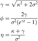
The short-rate dynamics in equation (8.17) were first suggested by Cox, Ingersoll and Ross in [55]. In the following, we indicate the CIR process in equation (8.17) as
When the parameters of the process satisfy the inequality
it is ensured that the process rt thus generated is always positive. Since the CIR model is of the mean-reverting type, both the expected value and the variance of rt tend to a constant value when time tends to infinity. In fact, at time t > 0, the average value of the CIR process CIR(κ, σ, θ, r0, t) is
which shows explicitly that the long-term average of the CIR process tends to the value θ. To prove the formula in equation (8.20), one might take the average on both sides of equation (8.17), and use the fact that Wt has zero average. One is left with an ODE with initial condition r = rs, leading to equation (8.20). With a similar technique, it can be shown that the variance of a CIR process is

Zero-coupon bonds
A closed-form formula is available for zero-coupon bonds, alternatively named discount bonds or discount factors, in the CIR model. For a process rt the moment-generating function over the time interval [t; T] is defined as
In the case of the CIR process in equation (8.17), m(q; t, T) is known in a closed-form formula,
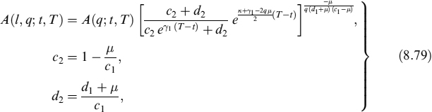
where the coefficients A(q; t, T) and B(q; t, T) are defined as

and with
The discount factor in the CIR model is then obtained from equation (8.23) when q = −1,
The explicit expression for the discount factor is given in CIR (see [55]):
with
and with ![]() .
.
Future and forward prices
Furthermore, futures and forward prices of zero-coupon bonds are available in closed-form formula in the CIR model.
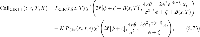
At time t, the future price3 of a future contract with maturity date s > t on a discount bond paying one monetary unit at time T > s is (see [53] for details):

where
The forward price of a forward contract to deliver at the maturity date s > t a discount bond paying one monetary unit at time T > s is (see [53])
The future price of the bond can be seen as its expected value at time s > t, under the risk-neutral measure:
On the other hand, the forward price of the bond can be considered as the expected value at time s > t under the forward risk-adjusted measure, also called the s-adjusted measure (see [34]), in which equation (8.17) becomes:
where the notation is the same as that introduced above. The forward price of the bond is then:
Probability distribution for a CIR process
In the CIR model, the process rt is characterized by a non-central chi-squared distribution. In particular, the probability distribution of the process in equation (8.18) is (see [55]):
where
and χ2(x; d, c) is the non-central chi-squared distribution, with d degrees of freedom and non-centrality parameter c.
It is also useful to give the CIR dynamics in the forward risk-adjusted measure, also called the t-adjusted measure: technically speaking, this is the measure under which the terminal payoff of a contract at time t is rescaled by dividing it by the value of a zero-coupon bond expiring at the time the probability distribution of the CIR process is:

where
As will be made clear in the models we will present, we will need both dynamics and distributions.
Options on bonds and interest rates
Following [55], the price of a European call option, with maturity s and strike K, on a zero-coupon bond with maturity T > s and with a short interest rate rt = CIR(κ, σ, θ, r0, t) is
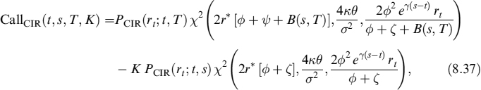
and with the quantity r* expressed in terms of the strike K by
Note that K = A(s, T)e−B(s,T)r* < A(s, T).
The value of the corresponding European put on the zero-coupon bond is found by put–call parity:
Although zero-coupon options are not actively traded in the market, equations (8.37) and (8.40) can be used to price much more common contracts such as cap and floor options on a discrete interest rate L(t, s, T) = LT(t), simply compounded and applied for a period starting at s and ending in T with strike rate X (e.g., a cap on a 3-month Eonia).4
The formula to evaluate a caplet with unit notional amount is:
A floorlet's value is given by the formula:
where the strike is
Let us now consider a cap or floor option, with maturity T and fixing schedule ti, i = {0, …, n − 1}, where n is the number of caplets or floorlets, and tn = T. The cap option is a sum of the caplets between fixing dates ti and payment dates ti+1, hence:

where we define the time intervals Ti = ti+1 − ti, and
Similarly, the floor is

Even if quotes on caps and floors on Eonia or OIS rates are not very liquid in the current financial markets, equations (8.41) and (8.42) can be useful to drive the distributions of discrete period rates that form the risk-free (Eonia or OIS) component of a Euribor or Libor fixing, if we model these as Ft(t) = Li(t) + Si(t), (i.e., as the sum of the risk-free rate plus a credit spread S). We will dwell more on this later on in this chapter.
Summing two CIR processes
It is useful to study some properties of the CIR process since we will exploit them heavily in the models we present in this book. We start by analysing the sum of two CIR processes.
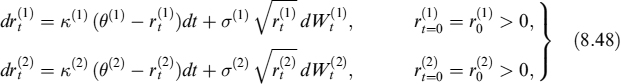
Let us consider two independent CIR processes,

We wish to know under which restrictions of the CIR parameters for ![]() and
and ![]() the process
the process ![]() is still a CIR process.5 To answer this, we consider the two CIR processes in the form given in equation (8.17),
is still a CIR process.5 To answer this, we consider the two CIR processes in the form given in equation (8.17),
so that the expression for drt is, considering the two processes ![]() and
and ![]() as independent,
as independent,

with the initial condition ![]() . We can write the expression for rt in equation (8.49) in the form
. We can write the expression for rt in equation (8.49) in the form
if we constrain the parameters as
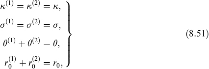
with the new Brownian motion Wt defined through
Summing up, if the CIR parameters for rt are defined as in equation (8.51), then
Multiplying a CIR process by a constant
We now consider how the process rt = CIR(κ, σ, θ, r0, t) is related to αrt, where α is a positive constant. For this, we multiply equation (8.17) by α,
or
Estimation of the CIR model using the Kálmán filter
Since we will also use the CIR model for risk management purposes and not only for pricing purposes (in which case we would just calibrate the model to market prices to infer risk-neutral parameters), we need a robust procedure to estimate the parameters according to historical prices. In this section, we outline a technique for estimating the parameters κ, θ and σ of the CIR model. For this, we use a maximum likelihood estimation based on the Kálmán filtering technique.
The basis of the procedure we present is to extract zero rates from market prices of zero-coupon prices: these prices are often embedded in coupon bonds that can be seen as portfolios of discount bonds. In the CIR model, the prices of a zero-coupon bond are related to the zero rate rt (here referred to as the latent variable) through the discount factor in equation (8.27). Indicating the bond maturity date by T, and setting
where P(t, T) is the market price of a discount bond. The relation between the latent variable and zt is
and is referred to as the observation equation. For the CIR model we have:
where A(t, T) and B(t, T) are the CIR factors defined in equation (8.28).
The Kálmán filter technique has become the standard tool for estimating the parameters of a short-rate model (not only the CIR model), given the term structure of a portfolio of bonds. Kálmán filters are based on time discretization of the equations describing the evolution of the interest rate rt (the latent variable) and of the bond price. If the time series of bond prices is considered from a date t0 to an end date t, we discretize the time interval [t0, t] by introducing the time step δ = (t − t0)/N, where N is the number of dates in the interval, and the dates are
Given the market price of the bond at time ti as pMKT(ti, t), we define
The discretized version of equation (8.57) is
where zi = zti, ri = rti, αi = αti and βi = βti. A second equation is obtained by considering the time evolution of the rate, according to equation (8.17),
where, for a CIR process, C = θ (1 − e−κδ) and F = e−κδ, while ωi is a Gaussian noise with mean equal to zero and variance equal to

With the Kálmán filter technique, equations (8.61) and (8.62) are simultaneously solved for ri and zi at step i, given the values of the variables at the i − 1-th step and the knowledge of zi from the market data at time ti, ![]() . As additional outcomes, the procedure produces values of the error
. As additional outcomes, the procedure produces values of the error ![]() , and the variance associated with the error Var zi. At each step, we construct the logarithm of the likelihood function
, and the variance associated with the error Var zi. At each step, we construct the logarithm of the likelihood function
The log-likelihood function of the process is the sum
The parameters κ, θ and σ are obtained by requiring that the function ![]() be maximized with respect to these parameters. In practical numerical codes, since minimization techniques are easier to implement, one looks for the parameters that minimize the function −
be maximized with respect to these parameters. In practical numerical codes, since minimization techniques are easier to implement, one looks for the parameters that minimize the function −![]() .
.
8.3.4 The CIR++ model
The CIR model is a parsimonious way to model the entire term structure of interest rates and also prevents negative values, in contrast to the Vasicek model. Nonetheless, it is often not rich enough to allow a perfect fit to observed market prices. On the other hand, when parameters are estimated from the historical time series, the model is unable in most cases to exactly reproduce observed market prices, even if they could be perfectly matched to them by means of single-time calibration.
In these cases it is convenient to extend the CIR model so as to allow perfect fitting to the initial term structure of (risk-free) interest rates, and a time-dependent deterministic extension is the easiest approach to adopt.
The CIR++ process
In the CIR++ model,6 the short-rate dynamics for rt are described as
where xt is a CIR process,
and ψt is a deterministic function that can be chosen so as to exactly match the initial term structure of interest rates. We denote the CIR++ model in equation (8.66) as
The price at time t of a zero-coupon bond expiring at T under a CIR++ process is (see [35]):
where ![]() is the discount factor defined in equation (8.27).
is the discount factor defined in equation (8.27).
The average value of the CIR++ process in equation (8.27) over the period [t, T] is
while, since ψt is a deterministic process, the variance of rt is given by the variance of the CIR process xt alone,
In a CIR++ model, we define the future in t, with expiry S and bond maturity T, as
where HCIR(t, S, T) is the future of the CIR process defined in equation (8.29).
Typically, the deterministic function ψt will be stepwise constant: we will see below how to fit it to actual market prices.
Options on bonds and interest rates
In the CIR++ model, the price of a European call option with maturity s and strike K on a zero-coupon bond with maturity T > s and interest rate rt = CIR++(ψt, κ, σ, θ, x0, t) is
where ϕ and ζ are as defined in equation (8.38), while
The value of the corresponding put on the European bond is found from the formula
Caps and floors in the CIR++ model are related to the call and put bond options as in equations (8.41) and (8.42).
8.3.5 The Basic Affine Jump Diffusion Model
An extension of the CIR model, which can be applied also to the CIR++ model, is the inclusion of jumps in the process of the short rate rt.7
A stochastic process Zt is a basic affine jump diffusion (bAJD) model if it follows the process
where Wt is a standard Brownian motion, and Jt is an independent compound Poisson process with constant jump intensity l > 0, so that jumps occur more frequently with increasing l. We assume that each jump is exponentially distributed, with mean μ > 0: the larger μ is the larger the size for a given jump. We also require κθ ≥ 0 in order for the process to be well defined. We indicate the process Zt in much the same way as the process in equation (8.76) as
Following [59] and [64], but with the notation as in [55], the moments of the bAJD in equation (8.77) are defined as
where
and where A(q; t, T) and B(q; t, T) are the CIR factors given in equation (8.24). In particular, all moments for the bAJD process reduce to the moments for the CIR process when either l = 0 or μ = 0, corresponding to the case in which either the intensity or the frequency of jumps is zero. In formulas, we have
as can be seen explicitly from the fact that when we set either μ = 0 or l = 0 in equation (8.79), the expression for m(1, q; t, T) reduces to m(q; t, T) in equation (8.23).
The discount factor in the bAJD model can be written in exponential form as
where
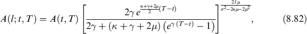
and where A(t, T) and B(t, T) are the CIR coefficients in equation (8.28).
8.3.6 Numerical implementations
We now focus on some numerical issues related to the CIR model and its extensions. More specifically, the CIR process has to be handled with care in its discrete version, used to simulate paths for the short-rate rt in Monte Carlo simulations.
8.3.7 Discrete version of the CIR model
Consider a short-rate factor rt described by a CIR process, as in equation (8.17), and a security that depends on rt. In order to evaluate the price of a contract at a future time s > t, or to simulate its cash flows, the value of rs has to be known. This can be done by numerically evolving rt using equation (8.17) in steps, from time t to time s. In greater detail let us introduce N discretization points ti, equally spaced by
so that
so that t0 = t and tN = s.
For the Brownian motion term dWt, we first note that
where the notation A ~ B means that the two distributions A and B are equivalent, and N0,1 is a Gaussian random variable of zero mean and variance equal to one. We generate a sample of N values ~N0,1 and call them Zi, so that
Setting r(ti) = rti, equation (8.17) is discretized as
Given the initial value r(t0) = r0, the entire solution is reconstructed in steps. The procedure in equation (8.87) goes under the name of the Euler scheme. A major failure of the Euler scheme is that it cannot guarantee that the process rt is always positive.
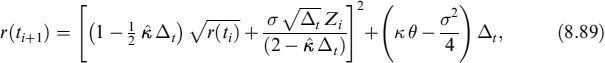
Of the various alternative schemes that have been proposed to mend this problem, [4] showed that the most suitable discretization for generating the process CIR(κ, σ, θ, r0, t) is

which provides a positive-definite process whenever the CIR condition in equation (8.19), 2κθ > σ2, is satisfied.
The same approach can be used to derive robust discretization for the forward risk-adjusted CIR process. A numerical implementation of the CIR process in this measure is (see [4]):
where ![]() .
.
We know that in the CIR++ model the short-rate rt is modeled as a sum of a stochastic term xt and a deterministic function ψt,
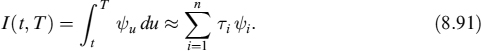
For the stochastic term, the same numerical procedures used for the CIR model can be employed. Instead, the deterministic function ψt can be modelled by a step function, with constant steps over some given time intervals. If the function is defined over the interval [t, T], we introduce a set of times Ti, i = {0, …, n}, with T0 = t and Tn = T, and we discretize the function ψTi = ψi with i = {1, …, n} so that ψi is constant over the corresponding step size Ti = Ti − Ti−1. An integral over [t, T] is then approximated by
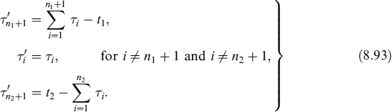
A little more care is needed if we wish to discretize an integral on the subinterval [t1, t2], with t < t1 < t2 < T. In this case, we first need to find the integer n1 for which Tn1 < t1 ≤ Tn1+1 and similarly the integer n2 for which Tn2 < t2 ≤ Tn2+1. The integral is then discretized as
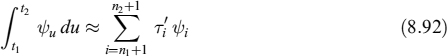
where
8.3.8 Monte Carlo methods
Consider a contract with maturity T and payoff H(r(T)). The value at time t of this contract is
where Et is the expectation value in the risk-neutral measure, while ![]() is the expectation value taken in the T-forward risk-adjusted measure (see Section 8.3.3). The discount factor PD(t, T) is obtained analytically, while the expected value of the payoff depends on the unknown value r(T) of the short rate at maturity.
is the expectation value taken in the T-forward risk-adjusted measure (see Section 8.3.3). The discount factor PD(t, T) is obtained analytically, while the expected value of the payoff depends on the unknown value r(T) of the short rate at maturity.
To compute the value of ![]() , we use the following Monte Carlo method. We generate p different paths of the discretized short rate, each path obtained by using the method in equation (8.89) for the forward risk-adjusted measure. In particular, for each path we obtain the value of the short rate at maturity and call it rj(T), with j ∈ {1, …, p}. The expectation value is approximated as
, we use the following Monte Carlo method. We generate p different paths of the discretized short rate, each path obtained by using the method in equation (8.89) for the forward risk-adjusted measure. In particular, for each path we obtain the value of the short rate at maturity and call it rj(T), with j ∈ {1, …, p}. The expectation value is approximated as
so that the price of the contract is

Pricing using a Monte Carlo method can be generalized to the case of path-dependent options. We consider the discretization of the short rate on the grid ti, {i = 0, …, N}, with t0 = t and tN = T, as discussed in Section 8.3.7. Defining
the price of the path-dependent contract is

The expectation value is computed by considering p realizations of the short rate in the T-forward measure. For a given realization j ∈ {1, …, p}, the value of the short rate at the discretized time ti is rj(ti). Setting
the price of a path-dependent contract is
8.3.9 Libor market model
The Libor market model (LMM) [31] approaches the problem by using forward rates that are directly observable in the market, such as Libor or Euribor fixings. While these rates could basically be considered as risk free up until 2008, in current markets they are actually traded as rates referred to default-risky countrparties, since even major banks are subject to this risk.
These considerations imply that the LMM can no longer be used to model Libor (or Euribor) fixing rates, but it is more appropriate to model Eonia forward rates, applying then a spread on these to derive the value of fixing rates. Anyway, for the moment we disregard this complication and we present the LMM in its standard version.
In the LMM, the quantities that are modelled are a set of forward rates rather than the instantaneous short rate or instantaneous forward rates. Consider a set of maturities {Ti|i = 1, …, N} describing the reset dates for traded caps or floors on the market. By including the additional date T0 = t, we define the time intervals Ti = Ti − Ti−1, i = {1, …, N} and the forward rates Li(t) observed at time t for the period (Ti−1, Ti]. In this model, the market has maturity TN = T.
Here, for each date i, we model the Libor rate Li(t) by a stochastic process under its forward measure, over the period [Ti−1, Ti]. Assuming that the Libor rate Li(t) is a martingale under the Ti-forward measure, we have
where σi(t) is the volatility of Li(t) at time t, and ![]() is an N-dimensional Brownian motion under the measure QTi, with instantaneous covariance matrix ρt.
is an N-dimensional Brownian motion under the measure QTi, with instantaneous covariance matrix ρt.
It is possible to link different Ti-forward measures with different values of i through a change of measure. As an example, we first consider the process for Li(t) in the T1-forward measure. Denoting by vi(t) the volatility of the zero-coupon bond price PD(t, Ti) at time t, we find
Forward rate agreement and caps&floors
In a forward rate agreement (FRA), at the inception time t, counterparties fix the expiry date S > t and the maturity of the contract T > S, to lock the interest rate over the period [S, T]. More specifically, at the maturity T, a payment with fixed interest rate K previously defined is exchanged in return for a floating payment based on the value of the Libor rate at time S, L(S, T). At time S, the value of the contract on a unit notional value is then
The value at time t of a FRA contract is
where the expectation value is taken in the T-forward measure, denoted by ![]() . It should be noted that the discount bond PD(t, T) is taken from a curve different from the Libor (or Euribor) one. This numeraire bond is calculated out of a risk-free interest rate curve: in the current financial environment the best approximation to a risk-free rate is considered the OIS (or Eonia) rate, so that PD(t, T) is in practice derived from the OIS (or Eonia) swap prices quoted in the market.
. It should be noted that the discount bond PD(t, T) is taken from a curve different from the Libor (or Euribor) one. This numeraire bond is calculated out of a risk-free interest rate curve: in the current financial environment the best approximation to a risk-free rate is considered the OIS (or Eonia) rate, so that PD(t, T) is in practice derived from the OIS (or Eonia) swap prices quoted in the market.
A forward rate agreed at time t is defined as the fixed rate to be exchanged at time T for the Libor rate L(S, T) so that the contract has zero value at time t. We denote the value of the forward rate as
When the Libor curve L(S, T) corresponds to the risk-free discount curve, we have an equality between the FRA rate and the forward rate computed out of the curve:
where P(t, ·) are zero-coupon bonds extracted by Libor fixing curves. However, as mentioned above, this has no longer been the case since 2008, and Libor curves are treated independently of the discount (OIS or Eonia) curves, see the discussion above.
Caps and floors are options of forward rates. We consider the set of payment dates {Ti|i = 1, …, N} and corresponding periods Ti = Ti − Ti−1, with i = 1, …, N, as discussed before, and we set T0 = S.
An interest rate cap is a contract in which the buyer receives a flow of payments at the end of each period in which the interest rate has exceeded an agreed strike price K. The price at time t of a cap option can be viewed as the sum of individual caplets,
At each time Ti, the option pays off the difference between the Libor rate and the strike X. Each caplet has a payoff
When the expectation value is taken in the Ti-forward measure, denoted by ![]() , we find
, we find
The pricing of floor options relies on similar techniques to those used for pricing caps. A floor is a contract in which the buyer receives payments whenever the interest rate falls below a strike price X. Decomposing the floor option as a sum of floorlets,
where each floorlet has the value in the Ti-forward measure of
The price of cap and floor options can be given in a closed-form formula using Black's formula [23], assuming that forward rates are lognormally distributed under the risk-neutral measure. The price of the cap option is

and the function BlSc(F, K, Σ) is as defined in Section 8.2. The value of ![]() is retrieved from the market quote σMKT,i for each i, as
is retrieved from the market quote σMKT,i for each i, as

and determines the price of the caplet through equation (8.112).
Swaps and swaptions
An interest rate swap (IRS) is a contract in which two parties agree to exchange one stream of cash flows against another stream. In a fixed-for-floating IRS, one party agrees to exchange a payment stream at a fixed interest rate K (the fixed leg of the contract) with a counterparty who in turn agrees to pay a flow of floating amounts (the floating leg).
In the following, we consider the term structure of payments for the floating leg given by the set {Ti|i = 1, …, n} defined above, together with the set ![]() , j = 1, …, nS, for the payment stream of the fixed leg of the contract. We define the time interval
, j = 1, …, nS, for the payment stream of the fixed leg of the contract. We define the time interval
and
for the floating leg. Usually, the floating rate is fixed at the beginning of each period and both payments are due at the end of the period.
At time Ti, the floating leg pays the Libor rate Li(Ti−1), where we set
while the fixed leg pays a fixed rate. The value of the swap contract at time t is
The forward rate swap S1,n(t) is the unique fixed rate for which the two payment flows from the floating and the fixed legs in equation (8.118) coincide,
Defining the weights
the price of the swap in equation (8.119) is written as a linear combination of Libor rates,
A European payer swaption is an option on interest rates swaps giving the right to enter an interest rate swap contract at a future time Te, when the fixed rate is K. In contrast, a receiver option gives the right to enter a receiver swap at time S. The payer swaption payoff at time S is
where we have defined the annuity
Using equation (8.119), we rewrite the swaption payoff as
Contrary to the cap option case, a swaption payoff cannot be decomposed into a sum of options on each period Ti. Moreover, in [35] it is shown that the price of a swaption depends not only on the evolution of each Libor rate, but also on their joint behaviour.
To price the payoff in equation (8.124), we consider the measure QC in which the annuity is the numeraire. In this measure, the formula for the price of a swaption of expiry S and maturity T is (see [89])
A closed-form formula is in theory unavailable. In practice, one may resort to the assumption of a lognormal distribution for the forward swap rate and thus obtain a pricing formula for payer swaptions of the type:

For a corresponding receiver swaption Swpt(t, Te, Tn, Se,n(t), K, σe,n, −1) we can resort to put–call parity.
Modelling the Libor rate with a spread over the forward rate
As already anticipated above, after the 2008 crisis, a spread Si(t) at time t between the risk-free rate (approximated by the OIS or Eonia rate) and the Libor or Euribor fixing rate is experienced in the market,
where Fi(t) = F(t, Ti−1, Ti) is the Libor (or Euribor) forward (FRA) rate and Fi(t) = F(t, Ti−1, Ti) is the risk-free OIS (or Eonia) forward rate. In general, we can decide to model using two stochastic processes two variables from Si(t), Fi(t) and Li(t), leaving the third determined by equation (8.127).
For swap rates, we use the fact that the swap s(t) is written in equation (8.121) as a linear combination of Libor foward rates. Writing the Libor rate as a sum of the forward rate plus a spread as in equation (8.127), we obtain
where we defined the processes

In particular, ![]() is a martingale under the measure QC. Following [89] and [68], the process
is a martingale under the measure QC. Following [89] and [68], the process ![]() can be treated, under generic assumptions, as a driftless process. In contrast, the pricing of the spread part
can be treated, under generic assumptions, as a driftless process. In contrast, the pricing of the spread part ![]() needs an additional assumption, since it depends on both the collection of spread rates Si(t) and on discount factors as a result of weights ωi(t). For this, we approximate the process as
needs an additional assumption, since it depends on both the collection of spread rates Si(t) and on discount factors as a result of weights ωi(t). For this, we approximate the process as
where we replaced the time dependence on the weight with the value at t0. With this approximation, ![]() is a martingale under QC and can be described, analogously to
is a martingale under QC and can be described, analogously to ![]() , by a driftless process.
, by a driftless process.
8.4 DEFAULT PROBABILITIES AND CREDIT SPREADS
In the credit risk literature, two different approaches to evaluating the probability of default have been developed; namely, the structural model and the reduced model. In a structural approach, the performance of the firm is governed by structural variables like the asset or the debt value, and a default is the result of poor operations of the firm. In reduced (or statistical) approach, the default intensity is modelled by a stochastic process, which might include jumps in the intensity of default λt.
The structural model and the reduced model are also referred to as endogenous and exogenous approaches, respectively, because in structural models the time of default is determined through the value of the firm, while in reduced models it is the jump of a stochastic process that determines bankruptcy.
We will mainly use reduced models, but we also quickly review structural models.
8.4.1 Structural models
In structural approaches, we model the structural variables of a firm (i.e., the assets and the debt value) using a stochastic or a deterministic process, in order to determine the time of default. Earlier literature on the subject includes [25], [91] and [24]. For example, in Merton's model, a firm defaults if its assets are below its debt when servicing the debt. In the Black and Cox model, a default occurs when the value V of the firm reaches a default boundary K.
Merton formula
Merton [91] proposed a model in which the firm value is treated as an option on the asset V. Suppose for simplicity that, at time t, the firm issues a bond with maturity T. We define the variables and parameters in Merton's model as in Table 8.1.
Table 8.1. Variables and parameters in Merton model
| Vt | Firm asset at time t |
| VT | Firm asset at time T |
| Et | Firm equity at time t |
| ET | Firm equity at time T |
| Bt | Value of the bond at time t |
| D | Debt repayment due at time t |
| σV | Volatility of the asset |
In the Merton model, the firm is financed through a single bond paying no coupons and a single equity issue. At any intermediate time t < s < T, the asset of the firm is
We assume that the asset follows the geometric Brownian motion described in Section 8.2,
where μ is the instantaneous expected rate of return, and Wt is a Brownian motion.
At time T, the firm repays its debt D. When VT < D, the firm defaults, and the value of the equity is zero. Conversely, if VT > D, the firm repays the debt and the equity has value ET = VT − D. At time T, the value of the equity is then
which resembles the payoff of a call option of the firm's asset Vt with strike price D. Using the Black–Scholes formula, we find the value of the equity at time t as
where r is the risk-free rate, N(x) is the cumulative probability distribution function for a normal distribution, and

Setting ![]() and using the notation in Section 8.2, we have
and using the notation in Section 8.2, we have
Although the structural approach is theoretically fascinating, it is hard to be satisfactorily calibrated to all available market data. The reduced-form approach we will sketch below is much more flexible, even if less linked to the microeconomic factors triggering the default event.
8.4.2 Reduced models
In a reduced-form approach, the event of default is modelled via an intensity of default λ. In this perspective, default intensities are modelled similarly to default-free interest rates, allowing us to use the same results and formulae previously described. In fact, it can be proved (see [62]) that, remarkably, defaultable bonds can be priced by adjusting the discount rate: this effective rate is the sum of the risk-free rate rt and the intensity of default λt, and both components can be treated with the mathematical tools we have shown before.
Given that the firm has not defaulted up to time t, the time of default T is defined as the probability of a default occurring in the next instant dt,
The intensity of default can be modelled differently as a
- constant (T is the first jump of a time-homogeneous Poisson process);
- deterministic function (T is the first jump of a time-inhomogeneous Poisson process);
- stochastic function (T is the first jump of a Cox process).
In particular, the second and third approaches can be used to model the term structure of credit spreads, and the third approach can be used to model credit spread volatilities.
The probability that the firm survives to time T, given we are at time t, equates
This definition is consistent with the expression in equation (8.137), by setting
In fact, equation (8.137) can be proved using the definitions in equations (8.138) and (8.139).
Modelling default intensities with a CIR process
We model the intensity of default by a CIR process
where we impose the additional constraint on the parameters 2κθ > σ2 in order to ensure positiveness of the process.8 At time t, the probability that the firm has not defaulted up to time T is given by equation (8.138) which, in the CIR model, can be written in the form of equation (8.27)
with the factors A(t, T) and B(t, T) as defined in equation (8.28). The corresponding probability of default is PD(t, T) = 1 − SP(t, T).
We can also suppose that the intensity of default is a CIR++ process, with the dynamics and the formula for the SP modified accordingly as described in Section 8.3.4.
Multiple defaults of correlated firms
For multiple issuers, we can assume that each default intensity process is the sum of an idiosyncratic component plus a common intensity of default. In this model, the default of the i-th issuer can be triggered by either the i-th idiosyncratic component or by the common component. Both the idiosyncratic and the common parts are described by independent CIR processes
where m is the total number of firms, and
The CIR process for the i-th firm is
where pi ∈ [0, 1] operates as a correlation of the i-th issuer with the probability of a common default: this approach to modelling is termed “affine correlation”.
The intensity is decomposed into an idiosyncratic term ![]() and a common intensity of default
and a common intensity of default ![]() . The idiosyncratic term is related to the probability that the default of the i-th issuer occurs independently of all other firms, while the process
. The idiosyncratic term is related to the probability that the default of the i-th issuer occurs independently of all other firms, while the process ![]() accounts for the probability that all firms default simultaneously. A common default affects the i-th issuer with a probability pi.
accounts for the probability that all firms default simultaneously. A common default affects the i-th issuer with a probability pi.
The sum of the two CIR processes in equation (8.144) does not automatically imply that λt,i is a CIR process. To find the constraints on the parameters, we first use the results in Section 8.3.3, to write the common process of default as
and (again from Section 8.3.3) the sum of the two CIR processes ![]() and
and ![]() is a CIR process λt,i if we impose the constraints in equation (8.51),
is a CIR process λt,i if we impose the constraints in equation (8.51),

For the correlated default intensities considered, the constraint in equation (8.19) reads
Likewise, the intensity process can follow the CIR++ process in equation (8.67). The deterministic part of λi,t is a function ϕi,t, and we have
8.4.3 Credit spreads
In Chapter 7 we quickly sketched how to set a fair credit spread for a loan contract, given the counterparty's probability of default and the loss given default. In this section we will try to show in more depth how to model credit spreads.
The modelling of credit spreads critically depends on assumptions made about recovery from the borrower's default: recovery is just complementary to loss given default. Let us assume that the loan has a face value of 1 which the borrower has to repay at expiry T, with (simply compounded) interest (r + s) × T, where r is the risk-free rate and s is the credit spread. The default can occur at any time between the evaluation time t = 0 and the expiry t = T, but is only observed by the lender at expiry when the repayment should be made.
There are different possible choices for recovery, two of which are most relevant for practical purposes:
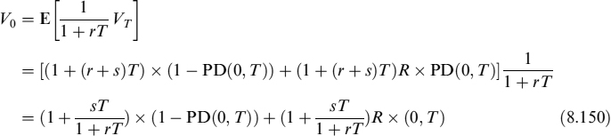
- Recovery of market value (RMV): upon the borrower's default, the lender recovers a fraction R = 1 − LGD of the market value of the loan. This means that the expected value VT at expiry (i.e., (1 + (r + s)T)) is:
At time 0, the expected value is:
Since the face value of the loan is 1 which is also the fair value it should have at inception when the amount is lent to the borrower (V0 = 1), from equation (8.150) we have:
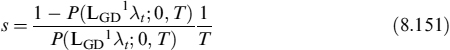
Setting LGD1 = LGD(1 + rT), recalling that

 , and using the approximation ec = 1 + c for small c, after a few manipulations we obtain:
where P(LGD1λt; 0, T) is the price of a zero-coupon bond expiring in T and with a discounting rate equal to LGD1λt. If λt follows a CIR model, it is possible to use formula (8.27) for a modified CIR process as shown in equation (8.54).
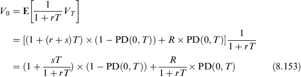
- Recovery of face value (RFV): upon the borrower's default, the lender recovers a fraction R = 1 − LGD of the face value (in our case, 1) of the loan. The expected value VT is:
At time 0, the expected value is:
Furthermore in this case, since V0 = 1, after a few manipulations we get:
Setting LGD2 = LGD + rT, we can write the spread as
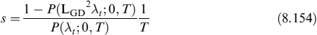
For loans with a short maturity and for a counterparty with a reasonably low PD (say, 3%), the denominator of both equations (8.151) and (8.154) can be set approximately equal to 1. Moreover, it is also easy to check that for small rT, LGD1 ≈ LGD2, so that for short-term loans, such as deposits in the interbank market, the two assumptions produce very similar spreads.
In conclusion, the credit spread between time t and T can be written as:
Equation (8.155) is a good approximation for both assumptions regarding recovery.
8.5 EXPECTED AND MINIMUM LIQUIDITY GENERATION CAPACITY OF AVAILABLE BONDS
Liquid assets are used to generate BSL and they can be considered as a component of the liquidity buffer, as seen in Chapter 7. We introduced the TSAA in Chapter 6 and showed how it is built and its connection with the TSLGC. We have left the problem of how to determine the future expected value of the assets, the unexpected minimum (stressed) values and the haircuts that can be applied unsolved. All this information is useful to the LGC because it is affected by the actual price of the assets on the balance sheet that can be used to extract liquidity and to match negative TSECCF.
In what follows we show how to monitor the LGC of one bond's holding and of a bond portfolio. Other assets, such as stocks, are less important as far as the LGC is concerned and they also require less sophisticated modelling. The main tool to monitor the LGC related to bonds is to build a term structure of minimum liquidity that can be generated at future dates within a chosen period at a given confidence level (e.g., 99%).
To build a term structure, we take the following steps:
- Divide the chosen period into a number of M subperiods;
- At the end of each subperiod tm compute the minimum value of the bond's holding or of the portfolio of bonds;
- Include the haircut either according to the approach outlined above or according to some predefined rules (e.g., ECB haircuts).
The building blocks we need to price the bonds and to compute the expected value and the stressed levels at future dates are:
- An interest rate model—we opt for the CIR++.
- A default model for multiple issuers—we opt for a reduced-form approach, with the default intensities depending on idiosyncratic and common factors (to account for the correlation between defaults and credit spreads). All intensities have CIR dynamics and a deterministic time function is added.
- A model for haircuts.
- A parameter to account for the specialness of single bonds.
8.5.1 Value of the position in a defaultable coupon bond
A defaultable coupon bond is a bond issued by an agent m that can default at some date in the future. Consider a bond held by the bank with the following characteristics:
- notional amount N;
- annual coupon rate c;
- coupon calendar {ti}, with coupon periods Ti = ti − ti−1;
- maturity T;
- loss-given-default rate LGD.
The value of the position in the bond with the specifics above is acquired at time t. We define the accrued time as the time between the last coupon payment and the acquisition,
The price of the coupon bond is
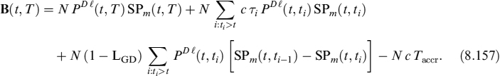
In the first line we have the sum of all coupon flows, discounted by the risk-free discount factors over the period [t, ti]. The third term accounts for the recovery paid in case of default, while the last term subtracts the accrual amount, which is the amount paid from the last coupon date to the time of acquisition. Obviously, setting N = 100 we get the market price of the bond.
We assume that the short rate follows CIR++ dynamics as in equation (8.66), so the function ![]() is given by the formula:
is given by the formula:
![]()
where ![]() is a bond-specific parameter to capture liquidity specialness and
is a bond-specific parameter to capture liquidity specialness and ![]() is defined in equation (8.27).
is defined in equation (8.27).
8.5.2 Expected value of the position in a coupon bond
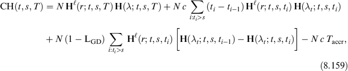
The expected value of the bank's position in a coupon bond can be easily computed, since it is the future price calculated according to the model we use for interest rates.9 We are interested in also computing the expected value net of the haircut, so we write the expected value of the position in a coupon bond as
where Ht(s) is the expected haircut at time s, see equation (8.166), while the future without including the haircut is
and
In this case ![]() is also given by the formula:
is also given by the formula:
![]()
where ![]() is the bond-specific parameter to capture liquidity specialness and HCIR++(r; t, s, T) is defined in equation (8.72).
is the bond-specific parameter to capture liquidity specialness and HCIR++(r; t, s, T) is defined in equation (8.72).
Equations (8.158) and (8.159) do not consider the possibility of default of the bond's issue between t and s. If the issuer goes bankrupt, the bank will not have a bond worth CH(t, s, T) but CH(t, s, T) − LGD, where LGD is the amount lost given the default. If we introduce the assumption the LGD = x%N, or a constant fraction of the par value of the bond, times the notional amount, then it is easy to consider the loss potentially suffered as well since in this case the expected value at time s would be:
CHDI(t, s, T) = CH(t, s, T) − LGDPD(t, s)
or, put into words, the expected value including the default event CHDI(t, s, T) is equal to the corresponding expected value without considering the default CH(t, s, T) minus the expected loss on default LGDPD(t, s).
The SP and the PD are modelled by a reduced-form approach where the default intensity of the n-th issuer is λt follows a CIR++ process too, so that formula (8.66) can also be used in this case:
Et[SPm(s, T)] = HCIR++(λt; t, s, T)
When a portfolio of bonds is considered, then the intensities of default are defined as in equation (8.148), where an idiosyncratic and common intensity and a deterministic time function ϕt appear.
We would like to stress the fact that for some issuers (typically sovereign) the PD can be zero and the bonds issued by them may even incorporate a liquidity discount (i.e., ![]() ), so that their yield could even end up being lower than a corresponding risk-free bond.
), so that their yield could even end up being lower than a corresponding risk-free bond.
8.5.3 Haircut modelling
At the present time t, the value H(t) of the haircut to be applied to the bond's market value is typically a function of the probability of default PD of the issuer. This can be inferred from the bond's price or from the rating the bond's issuer has.
An approach based on the maturity T and credit rating has also been adopted by the ECB.10 For a given maturity, the bond can be Step 1 and 2 if the harmonized rating is between AAA to A−, so that it has a haircut depending on the maturity and the category H1; otherwise, the bond can be Step 3 if the rating is between BBB+ and BBB−, with a haircut H2; finally, the bond can be out of the eligible set that is accepted by the ECB as collateral and implicitly has a haircut H3 = 100%, since no liquidity can be extracted from it by a repo transaction with the central bank.
A similar approach can be followed when simulating the haircut of a bond, since in the end a bond can always be pledged in a collateralized loan with the ECB. For the haircut to be applied at a future time s, we model H(s) with a three-step function. Given two levels of the survival probability in the next period (say, 1 year) K1 and K2 < K1, the bond at time s is Step 1 and 2 (first quality according to the ECB's classification) if its default probability is below 1 − K1; it is Step 3 if its default probability is between 1 − K1 and 1 − K2; finally, it is considered ineligible if its default probability is higher than 1 − K2.
We adopt a reduced-form approach to model the default probability of the issuer, and we assume that the default intensity follows a CIR process as in equation (8.140), using equations (8.139) and (8.141):
![]()
where ϕt is a deterministic function and the CIR stochastic function is defined as
![]()
We can derive the probability that the bond falls in the first, second or third of the groups described above. In particular, the probability at time t that the bond at time s falls in the first (Step 1 and 2) group is
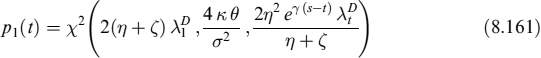
where, ![]() . We define the parameters
. We define the parameters
and, by making the trigger K1 equal to the discount factor on [s, s + THor] computed from the CIR++ intensity λt, we find
where THor sets the default time horizon from the time at which we compute the haircut. We can set THor = 1 year, for example, or we can link the function to a longer term PD by setting THor = 5 years.
Similarly, the probability that the PD at time s is between 1 − K1 and 1 − K2 is
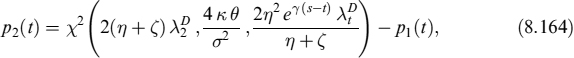
with
Finally, the probability that the PD lies above 1 − K2 is p3(t) = 1 − p1(t)− p2(t).
The expected haircut at time s is then
Since we presented a model for stochastic default intensities in Section 8.4, we can use it to model stochastic haircuts evolving in the future according to changes in the issuer's PD.
8.5.4 Future value of a bond portfolio
We are able to calculate the expected value of a bond's position at future dates; it is not a major problem to compute the expected value of a portfolio of bonds as well, since it is the sum of the single expected values. We are interested in finding a way to determine which is a stressed minimum level that the bond, or the portfolio of bonds, can reach at different dates in the future at a defined confidence level, say, 99%. In this case the correlation between issuers plays a major role in reducing the distance between the expected and the stress level, or the unexpected variation of the bond or portfolio of bonds.
8.5.5 Calculating the quantile: a Δ − Γ approximation of the portfolio
We consider a portfolio comprising NB bonds and issued by Nf issuers. For each issuer i, there are Ni bonds in the bank's portfolio; each bond's position has value Bi(t, Tj) and expected CHi(t, s, Tj), 1 ≤ j ≤ Ni. For numerical reasons, if a liquidity discount for the i-th bond exists (i.e., ![]() ), then the corresponding value of the process λi,t for the i-th issuer is theoretically zero, although we set it to 1e-10, and so is the value of the function ϕt.
), then the corresponding value of the process λi,t for the i-th issuer is theoretically zero, although we set it to 1e-10, and so is the value of the function ϕt.
Defining the vector of intensities11
the expected value of the position for all bonds at time s is
We perform a Δ − Γ approximation of the value of the portfolio at time s, around the value Ys, as
The vector Δ and the symmetric matrix Γ are computed by taking the numeric first and second derivatives of the portfolio V(Yt) with respect to rt and λi,t. We recall that, given a function f(x, y), the first derivative along x is approximated as
the second derivative along x is
and the mixed derivative is

The dimension of Δ and the rank of Γ both equate to Nf + 1. Setting
and
we rewrite equation (8.169) as
This assumes that Ys has a Gaussian distribution, with mean M = (Mr, Mλ)T and a covariance matrix
For the CIR++ processes in equation (8.67), and the intensity ![]() decomposed as in equations (8.142), and (8.143), at time s we have the mean
decomposed as in equations (8.142), and (8.143), at time s we have the mean
while the covariance matrix is
We recall that ![]() and
and ![]() . For Nf firms, the dimension of the vector M and the rank of the covariance matrix Ω are both Nf + 1.
. For Nf firms, the dimension of the vector M and the rank of the covariance matrix Ω are both Nf + 1.
Now we are able to compute the value of the quantile v for which there is a probability p = P(V(Ys) < v) that the value of the portfolio at time s > t falls below v. To obtain P(V(Ys) < v), we first Fourier-transform V(Ys), defining the function
The probability relates to ϕ(u) according to the formula of Gil-Pelaez [72],
To perform the integration numerically, we first rewrite it as

then we introduce a grid with equally spaced abscissae u → uj = (j + 1/2)δx, with step size δx and j running from one to an integer K. The integral is then truncated from zero to K δx, and equation (8.184) is approximated by

Fixing the time horizon s and the probability p that the portfolio falls below the level v, we invert equation (8.183) to obtain the quantile v; namely, we invert
To find v numerically, we use a bisection method.
Since v only accounts for the market value of the portfolio of bonds given that no default of the issuers occurs during the period [t, s], if we are interested in considering the quantile that also includes the losses suffered if one or more issuers go bankrupt we can compute the expected loss for the portfolio in the event of defaults,

so that the quantile with default included is:
The minimum level of a portfolio of bonds at the 99% c.l. corresponds to the first quantile of the distribution and is derived as described above.
8.5.6 Estimation of the CIR++ model for interest rates
To estimate the parameters of the process xt in equation (8.66) (the process for the instantaneous interest rate) from market data, we can consider a series of discount factors bootstrapped from the Eonia swap quotes. We mentioned above that the Eonia rate can be considered virtually risk free, since it embeds the credit risk related to lending money to a bank for one day; moreover, swap rates with the Eonia rate as the underlying are assumed to be fully and continuously margined, so that counterparty credit risk is almost totally eliminated. In the end the Eonia rate and swaps on Eonia can be supposed to be the contracts from which it is possible to extract the risk-free term structure of interest rates.
The estimation involves two steps:
- Estimate the parameters of the process xt with the Kálmán filter, as explained in Section 8.3.3.
- Calibrate a time-dependent function ψt with the market data of each date of the time series, so as to have a best fit of the model.
Let us now provide a practical example of estimating the parameters using real market data.
Example 8.5.1. We consider a panel of bootstrapped discount factors, obtained from the Eonia swap rate quotes with maturities given in Table 8.2. The time series of the term structures of the swap rates is considered in the period running from 31/12/2010 to 4/6/2012. We plot the 1W, 1Y, 5Y, 10Y and 30Y swap rates in Figure 8.1.
Table 8.2. Maturities of Eonia swap rates used in the estimation procedure
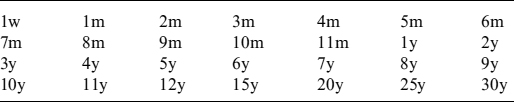
Discount factors on the same set of maturities as in Table 8.2 are derived for each date and used for the estimation with the help of the Kálmán filter technique, obtaining the results in Table 8.3.
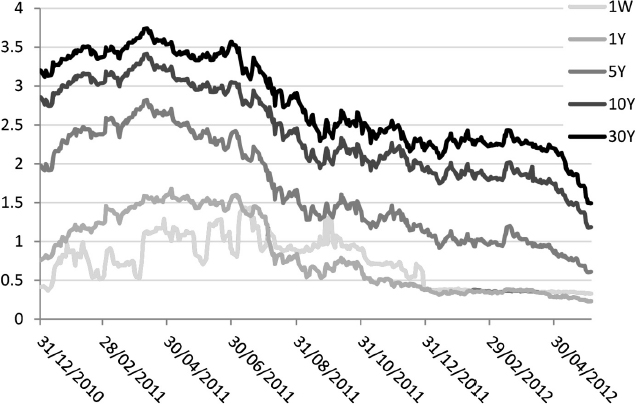
Figure 8.1. Eonia swap rates from 31/12/2010 to 4/6/2012
Table 8.3. Values of the parameters of the CIR model for the zero rate, obtained using the Kálmán filtering technique described
| Parameter | Value |
| κr | 0.08178 |
| θr | 6.23% |
| σr | 10.1% |
The deterministic function in equation (8.66) is found by requiring, for any date tm in the panel data, a perfect match between the swap rate data of the time series with maturity Ti, Pdata(tm, Ti), and the value of the discount factor P(x; tm, Ti) from equation (8.69), imposing
PCIR(x; tm, Ti) is known since we have already calibrated the CIR process for xt (we approximate the value of x0 using the Eonia overnight). We use the other Nϕ = NEonia − 1 series of Eonia maturities to construct the function ψt. We define a series of Nϕ time steps ΔTi as
![]()
We ignore the first value T1 that refers to the maturity at one week. Assuming that ψt is a step function, of step size ΔTi, the integral of ψt is
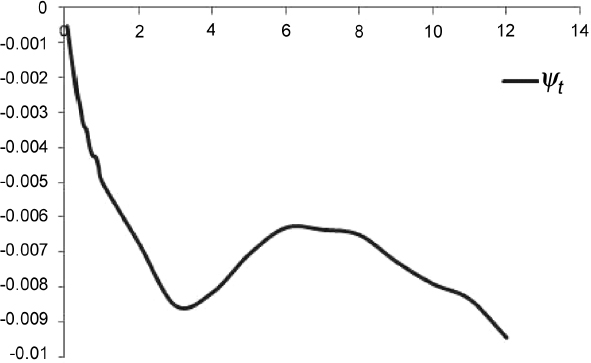
Figure 8.2. The function ψt, obtained with the method described in the main text, as a function of maturity
the values for ψt are then built iteratively. The first value of the step function is
while the i-th value is

Note that, if there are M days of observation, this technique results in M step functions ψt.
Example 8.5.2. We use the panel data described in Example 8.5.1 with the calibrated parameters for the zero rate in Table 8.3 to construct the function ψt. We show a plot of ψt as a function of maturity in years in Figure 8.2.
8.5.7 Estimation of the CIR++ model for default intensities
In order to calibrate the parameters describing the intensities of default, we need to modify somewhat the Kálmán filter procedure described in Section 8.3.3 for the zero rates. Intensities of default are calibrated using a time series of coupon bonds, in which we consider a total of NB coupon bonds and Nf issuers.
The number of CIR processes to be calibrated is Nf + 1, corresponding to the number of idiosyncratic processes Nf (one for each firm), plus the common process. For each day t, we store this information into the vector yk,t, where the first entry y0,t is for the common intensity of default, and the remaining Nf entries are for each idiosyncratic process. The total number of parameters to be calibrated is
Table 8.4. Specifics for the bonds issued by Italy, France and Spain
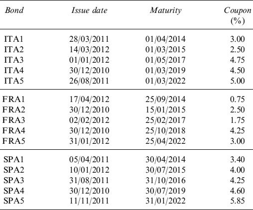
corresponding to κ, θC, σC plus pi and ![]() for each firm i.
for each firm i.
Example 8.5.3. We consider a portfolio of 15 bonds, issued by Italy (ITA), France (FRA) and Spain (SPA), respectively, over the period from 31/12/2010 to 25/05/2012 and with the specifics in Table 8.4. For each bond, we take into account the time series of prices from the beginning of the period, or the issue date if later, to the end of the period. We estimate the values of the parameters from the time series of bond prices using the Kálmán filter technique, obtaining the results in Table 8.5. In Figure 8.3, we plot the intensity of default λt for each issuer ITA, FRA, SPA, over the period 31/12/2010 to 25/5/2012, obtained by the Kálmán filter.
Having calibrated the parameters of the CIR processes commanding the intensity of default of each issuer, we need to calibrate at the reference time t = t0. We choose to use the model of the value of the intensity λ0,i for the i-th issuer, which can be decomposed into an idiosyncratic term ![]() and a common term
and a common term ![]() as
as
Defining the total number of bonds in the portfolio NB as in equation (8.168), we construct the function
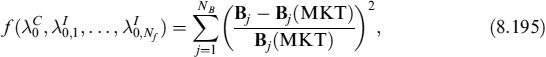
Table 8.5. Values of the parameters of the CIR model for the intensity of default process for the three issuers Italy, France and Spain, obtained with the Kálmán filtering technique
| Parameter | Value |
| κr | 0.0465 |
| θC | 1.1257% |
| θITA | 11.477% |
| θFRA | 4.974% |
| θSPA | 11.835% |
| σC | 6.634% |
| PITA | 0.883 |
| PFRA | 0.668 |
| PSPA | 0.867 |
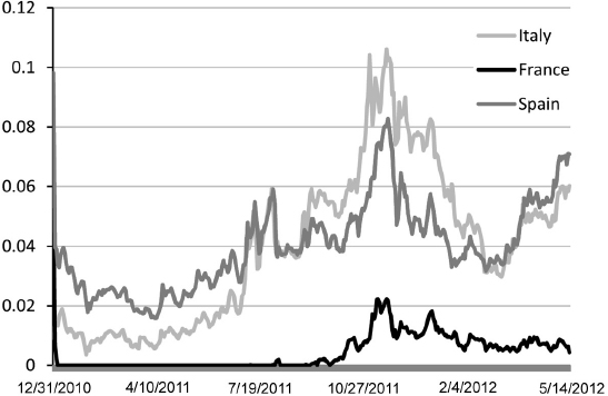
Figure 8.3. The value of the default intensity as a function of time, for the three issuers Italy, France and Spain, obtained from the Kálmán filter technique
where Bj(MKT) is the market price for the j-th bond and Bj is the model price for the same bond according to equation (8.157). At this stage, we have set to zero the values of the functions ϕi,t for all firms, while we consider the calibrated function ψt for the zero-rate process. The values of ![]() and
and ![]() are found by requiring that the above function be minimized.
are found by requiring that the above function be minimized.
After estimating the initial values λ0,i, for each issuer i, we model the time-dependent ϕi,t with a step function of step size ΔTϕ, for a total of Nϕ steps. For the i-th issuer, Nϕ is fixed by the bond with the longest maturity, say TJ, so that
where t0 is the last day considered and [x] is the integer part of x.
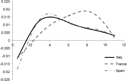
Figure 8.4. The value of the function ϕt as a function of time, for the three issuers Italy, France and Spain
The function ϕi,t is calibrated to the market data by a least squares procedure. We consider the function
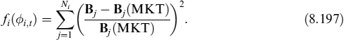
In equation (8.197), the sum runs over the Ni bonds issued by the i-th firm, Bj is the price of the j-th defaultable coupon bond according to equation (8.157) and Bj(MKT) is the corresponding market price for the same bond.
We demand the function fi(ϕi,t) to be minimized with respect to ϕt, under the additional constraint that the second derivative of ϕi,t be minimized at each step as well.
Example 8.5.4. We consider the market bond prices of the portfolio described in Example 8.5.3, on the reference date 25/5/2012. Using CIR parameters for the zero rate and the default intensities in Tables 8.3 and 8.5, and using the function ψt obtained in Example 8.5.2, we obtain the model price in equation (8.157) for each issuer as a function of ϕi,t for that issuer. Using the methods described in this section, we calibrate the functions ϕi,t with the market data, obtaining the results shown in Figure 8.4.
The model bond prices resulting from the estimated parameters and the deterministic function are shown in Table 8.6: for each bond we also show the theoretical price obtained only by the CIR component of the default intensity model and the price obtained by adding the time-dependent function.
Example 8.5.5. We consider the market bond prices of the portfolio described in Example 8.6.1, on the reference date 4/6/2012. Using CIR parameters for the zero rate and the default intensities in Table 8.3 and 8.21, and using the function ψt obtained in Example 8.5.2, we obtain the model price in equation (8.157) for each issuer as a function of ϕi,t for that issuer. Using the methods described in this section, we calibrate the functions ϕi,t with the market data, obtaining the results shown in Figure 8.5.
Table 8.6. Model bond prices in Example 8.5.3
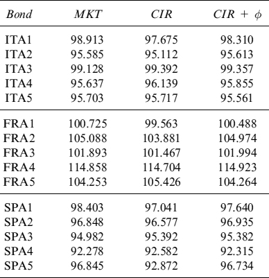
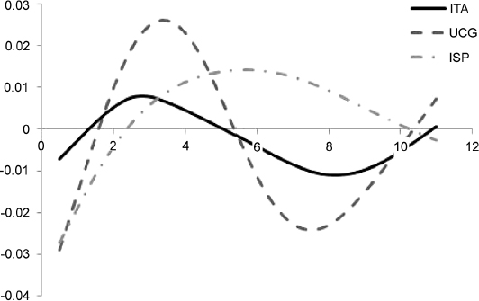
Figure 8.5. The value of the function ϕt as a function of time, for the three issuers Italy, Unicredit and Intesa Sanpaolo Bank
Finally, we need to compute the bond-specific parameter ![]() to perfectly match market bonds priced with model prices obtained with the estimated parameters. The value of
to perfectly match market bonds priced with model prices obtained with the estimated parameters. The value of ![]() can easily be found with a numerical procedure like the Newton–Rahpson method or bisection.
can easily be found with a numerical procedure like the Newton–Rahpson method or bisection.
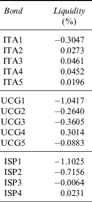
Example 8.5.6. We refer to the portfolio described in Example 8.5.3. Using the method described in this section, we find the liquidity parameter for each bond as in Table 8.7.
Table 8.7. Liquidity parameters for each bond considered in Example 8.5.3

It is worthy of note that not all issuers have to be given a default probability. In some cases the bond prices show that the theoretical price can match market quotes only if the default intensity is set equal to zero and the process does not depart from this value. It is also likely that in these situations a liquidity premium (i.e., ![]() ) is implied in market quotes, as we will see in the next example.
) is implied in market quotes, as we will see in the next example.
Example 8.5.7. To the portfolio in Example 8.5.3 we add five additional bonds issued by Germany (GER). the specifics for the GER bonds are given in Table 8.8. Since the market price of these bonds is above the price obtained using the bond formula in equation (8.157) with the intensity parameter λt = 0, there is only a liquidity premium to be attached to these bonds. We obtain the liquidity parameter ![]() for each bond in Table 8.9.
for each bond in Table 8.9.
Table 8.8. Specifics for the GER bonds considered
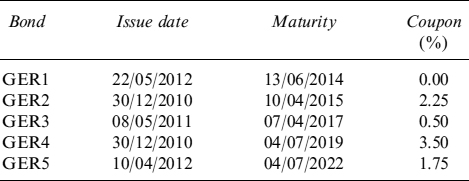
Table 8.9. Liquidity parameter for the GER bonds in Table 8.8
| GER1 | −0.2371% |
| GER2 | −0.2195% |
| GER3 | −0.2297% |
| GER4 | −0.1140% |
| GER5 | −0.0257% |
Example 8.5.8. We consider the portfolio of bonds with the specifics in Table 8.20. Using the method described in this section, we find the liquidity parameter for each bond as in Table 8.10.
Table 8.10. Liquidity parameters for each bond considered in Example 8.6.1
8.5.8 Future liquidity from a single bond
We now have all the information to forecast the expected and minimum (at a given confidence level) liquidity that can be extracted form a bond: in fact, we can obtain liquidity as analysed in Chapter 6 when describing the TSAA, by selling or pledging the bond in a collateralized loan (which is in practice the same as repoing it).
If we know the expected and minimum levels of the price, with or without the haircut, we can build a term structure of liquidity that can be generated by the bond by adding this information to the TSAA. In the next example we show how the model we have calibrated in this section can help produce these data.
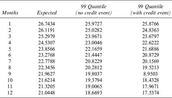
Example 8.5.9. We consider a portfolio of EUR30 million notional containing only the bond issued by Italy maturing in 2017, see Example 8.5.3. We compute a term structure of expected price levels and of minimum levels at the 99% quantile over a period of one year, in monthly steps. We also compute this stressed minimum level by considering and excluding the default event: in the latter case the intensity of default affects the price but does not trigger any jump event. When a haircut is not applied, we obtain the values in Table 8.11 and Figure 8.6 indicating the different levels of future liquidity.
Table 8.11. Term structure of expected and minimum (99% c.l.) levels of liquidity (million), with and without credit event, generated by EUR30 million invested in the bond issued by Italy and maturing in 2017. The term structure is considered over one year, in monthly steps. No haircut has been applied
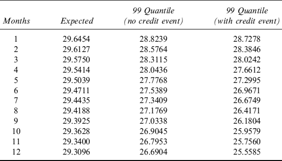
The information contained in Table 8.11 can be used when building the TSAA and the TSLGC to estimate how much liquidity can be obtained by selling the bond in the next year.
The same type of analysis can be conducted by including the haircut so as to forecast the potential liquidity obtainable by repo transactions. We assume that the haircuts are determined by an approach such as the one explained above, and that the bond in the Step 1 and 2 group of the PD over one year is below 5%, whereas it falls in the Step 3 group when the PD is below 15% (above 15% it is no longer eligible for repo transactions). We obtain the term structure of expected and stressed levels at the 99% c.l. in Table 8.12 and Figure 8.7.
We can also set the trigger for the passage from Step 1 and 2 to Step 3 at lower PD levels. For example, we can leave the first trigger at 5% PD over one year and lower the second trigger to 7.5%. In this case we obtain the term structure in Table 8.13 and Figure 8.8.
8.5.9 Future liquidity from more bonds
The framework we have designed can also cope with a portfolio of many bonds with different maturities: in this case the bank can take advantage of the diversification effects that can be attained by buying bonds with different exposures to interest rates and to the evolution of the PD. It is clear that in this case the TSAA needs to be built while considering the aggregated position the bank has on a single issuer as well, since information on just one bond can be useful but is only a small part of the entire picture of the BSL.
Table 8.12. Term structure of expected and minimum (99% c.l.) levels of liquidity (million), with and without credit event, generated by EUR30 million invested in the bond issued by Italy and maturing in 2017. The term structure is considered over one year, in monthly steps. We applied a haircut with triggers at 5% and 15% for the PD over one year

Table 8.13. Term structure of expected and minimum (99% c.l.) levels of liquidity (million), with and without credit event, generated by EUR30 million invested in the bond issued by Italy and maturing in 2017. The term structure is considered over one year, in monthly steps. We applied a haircut with triggers at 5% and 15% for the PD over one year
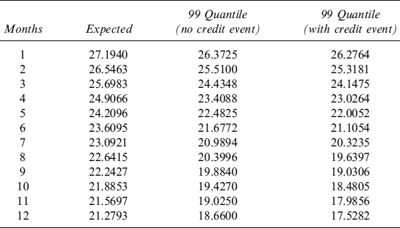
Example 8.5.10. Consider a portfolio of EUR30 million, equally distributed among the five bonds issued by Italy and with the specifics given in Example 8.5.3. The term structure of expected price levels and of minimum levels at the 99% quantile over a period of one year, in monthly steps, can be computed with the approach described in the main text. In this example we also compute this stressed minimum level by considering and excluding the default event, as in Example 8.5.9. When a haircut is not applied, we obtain the liquidity that can be generated by selling the portfolio at future dates, both at an expected and at a minimum level (99% c.l.), as shown in Table 8.14 and Figure 8.9.
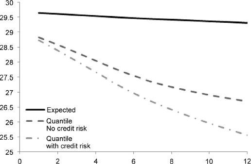
Figure 8.6. Term structure of expected and minimum (99% c.l.) levels of liquidity, with and without credit event, generated by EUR30 million invested in the bond issued by Italy and maturing in 2017, as in Table 8.11
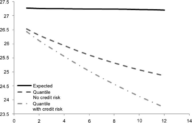
Figure 8.7. Term structure of expected and minimum (99% c.l.) levels of liquidity, with and without credit event, generated by EUR30 million invested in the bond issued by Italy and maturing in 2017, as in Table 8.12
Moreover, bond portfolios can be repoed out, so we can compute the expected and minimum liquidity by including the haircuts too. As in Example 8.5.9, we assume two levels of PD triggering the passage from the ECB's Step 1 and 2 to Step 3 at 5%, whereas above 15% the bonds are no longer eligible for repo transactions. Table 8.15 and Figure 8.10 show the results.
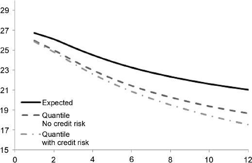
Figure 8.8. Term structure of expected and minimum (99% c.l.) levels of liquidity, with and without credit event, generated by 30 million euros invested in a portfolio of five bonds issued by Italy, as in Table 8.13
Table 8.14. Term structure of expected and minimum (99% c.l.) levels of liquidity (million), with and without credit event, generated by EUR30 million invested in a portfolio of five bonds issued by Italy and maturing. The term structure is considered over one year, in monthly steps. No haircut has been applied

Haircuts play a major role on the liquidity that can be obtained by repo transactions when a portfolio of bonds is also considered. In fact, when a higher haircut is triggered with higher probabilities, the minimum liquidity is strongly affected as shown in Table 8.16 and Figure 8.11: in this case triggers are set at 5 and 7.5% of the PD at one year.
Table 8.15. Term structure of expected and minimum (99% c.l.) levels of liquidity (million), with and without credit event, generated by EUR30 million euros invested in a portfolio of five bonds issued by Italy and maturing. The term structure is considered over one year, in monthly steps. We applied a haircut with triggers at 5% and 15% for the PD over one year
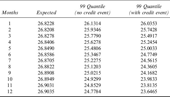
Table 8.16. Term structure of expected and minimum (99% c.l.) levels of liquidity (million), with and without credit event, generated by EUR30 million invested in a portfolio of five bonds issued by Italy and maturing. The term structure is considered over one year, in monthly step. We applied a haircut with triggers at 5 and 7.5% for the PD over one year
The BSL needs to be considered at an aggregated level when bonds are issued by several debtors as well. In this case we should also take into account the correlations between the probabilities of default that affect not only the losses suffered by the holder (the bank in our case) when the issuers go bankrupt, but also the price of the bonds in the portfolio.
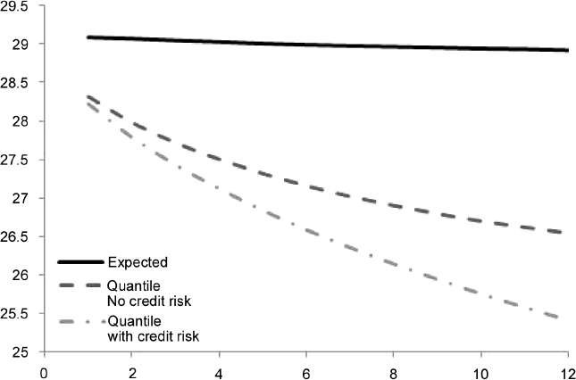
Figure 8.9. Term structure of expected and minimum (99% c.l.) levels of liquidity, with and without credit event, generated by EUR30 million invested in a portfolio of five bonds issued by Italy, as in Table 8.14

Figure 8.10. Term structure of expected and minimum (99% c.l.) levels of liquidity, with and without credit event, generated by EUR30 million invested in a portfolio of five bonds issued by Italy, as in Table 8.15
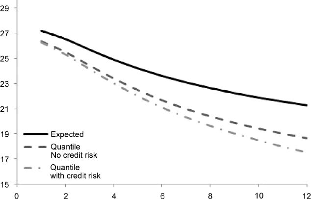
Figure 8.11. Term structure of expected and minimum (99% c.l.) levels of liquidity, with and without credit event, generated by EUR30 million invested in a portfolio of bonds issued by Italy, as in Table 8.16
The model we have introduced is capable of accounting for the correlation by using the composite CIR++ process: this correlation affects the liquidity that can be generated by the portfolio in two ways:
- Prices are more correlated if the default intensities of the issuers are more correlated.
- The haircuts of the bonds increase jointly with higher probability if the intensities are more correlated, since they are linked to the credit rating and we assumed that this is dependent on the probability of default, as explained above.
In both cases the liquidity that can be generated at future dates by the portfolio of bonds is smaller.
Example 8.5.11. We consider a portfolio of EUR30 million, equally distributed among 20 bonds, 15 of which are those considered in Example 8.5.3, while the other 5 are the GER bonds in Example 8.5.7. We compute the term structure of the expected and minimum liquidity (99% c.l.) that can generated by the portfolio. We start by considering the case the when the portfolio is sold, so we exclude the haircuts. The results are in Table 8.17 and Figure 8.12.
If the bank wants to compute the expected and minimum liquidity that can be extracted from the bond portfolio by repo transactions, the haircut has to be included. We assume that the levels at which the PD triggers passages between haircuts, modelled on the ECB's approach as explained in the main text, are set at 5 and 15% for all issuers. We obtain the term structure of liquidity in Table 8.18 and Figure 8.13.
When higher haircuts are more likely, such as when they are triggered by PD levels set at 5 and 7.5%, we obtain the term structure of liquidity in Table 8.19 and Figure 8.14.
Table 8.17. Term structure of expected and minimum (99% c.l.) levels of liquidity (million), with and without credit event, generated by EUR30 million invested in a portfolio equally distributed among 20 bonds issued by ITA, GER, FRA, SPA. The term structure is considered over one year, in monthly steps. No haircut has been applied
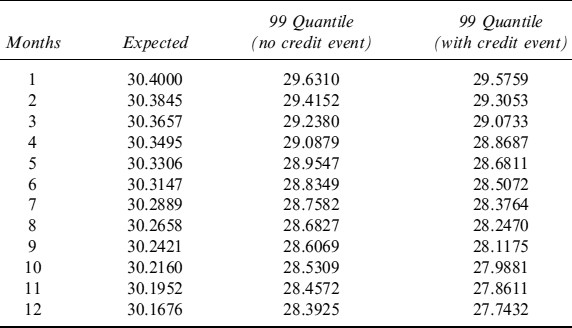
Table 8.18. Term structure of expected and minimum (99% c.l.) levels of liquidity (million), with and without credit event, generated by EUR30 million invested in a portfolio equally distributed among 20 bonds issued by ITA, GER, FRA, SPA. The term structure is considered over one year, in monthly steps. We applied a haircut with triggers at 5 and 15% for the PD over one year

8.6 FAIR HAIRCUT FOR REPO TRANSACTIONS AND COLLATERALIZED LOANS
In the previous section we introduced a tool to monitor the LGC of a portfolio of bonds held by the bank. In the case of liquidity generated by repo transactions, we have modelled the haircut to apply to the market price of the bonds following the approach adopted by the ECB since, first, the central bank is the main counterparty for European banks12 and, second, because the ECB's haircuts are often used as a guide to set haircuts for transactions not involving the central bank itself.
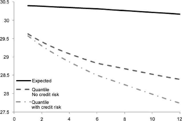
Figure 8.12. Term structure of expected and minimum (99% c.l.) levels of liquidity, with and without credit event, generated by EUR30 million invested in a portfolio of bonds issued by ITA, GER, FRA, SPA, as in Table 8.17
Table 8.19. Term structure of expected and minimum (99% c.l.) levels of liquidity (million), with and without credit event, generated by EUR30 million invested in a portfolio equally distributed among 20 bonds issued by ITA, GER, FRA, SPA. The term structure is considered over one year, in monthly steps. We applied a haircut with triggers at 5 and 7.5% for the PD over one year
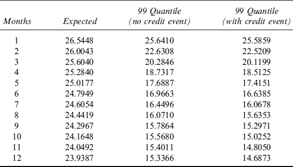
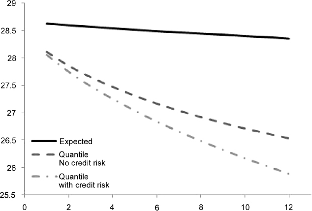
Figure 8.13. Term structure of expected and minimum (99% c.l.) levels of liquidity, with and without credit event, generated by EUR30 million invested in a portfolio of bonds issued by ITA, GER, FRA, SPA, as in Table 8.18
Nonetheless, we would like to design an approach to set fair haircut levels for repo transactions and collateralized repos which is somehow different and possibly more robust than that devised by the ECB. In fact, one of the main flaws of the ECB's approach to set haircuts is that it does not consider wrong-way risk in any way: this increases the probability of there being a joint default of the counterparty borrowing money in the deal and the issuer of the bond pledged as collateral. This situation clearly makes the collateral lose its risk mitigation feature and the credit risk to the lender approaches that of a non-collateralized loan.
We would like to stress the fact that wrong-way risk is very common for the following reason: collateral bonds are often Treasuries issued by the government of the country of the borrower bank. Typically, there is a strong correlation between the credit spreads (which reflects the PDs) of the Treasuries and the banks, for the circular fact that banks have huge quantities of Treasury bonds on their balance sheets to build the liquidity buffers. So, when crises occur with sovereign debts, such as the one experienced in 2011–2012 in Europe,13 the PD of the banks of the countries under pressure increase as a result of the higher probability of default of the sovereign debt they hold as assets. Banks of countries such as Greece, Spain, Portugal, Ireland and Italy pay high credit spreads over the risk-free rate (however we define it) because they are perceived as high risk for the Treasury bonds they hold (and for the more general country risk).
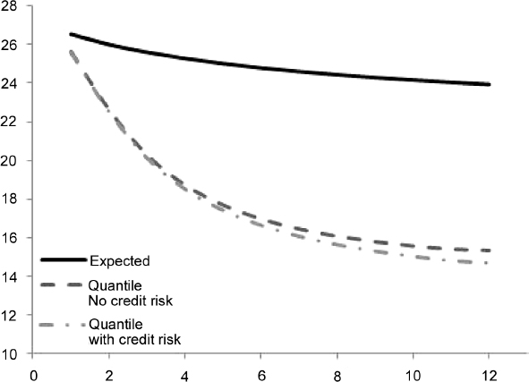
Figure 8.14. Term structure of expected and minimum (99% c.l.) levels of liquidity, with and without credit event, generated by EUR30 million invested in a portfolio of bonds issued by ITA, GER, FRA, SPA, as in Table 8.19
The framework we have introduced above is rich enough to effectively cope with this problem as well. Assume that counterparty d posts a portfolio of NB bonds, issued by Nf issuers as collateral for a loan (or for a repo transaction). For each issuer there are Ni bonds in the portfolio: the notional of the loan at inception is the same as the value of the portfolio minus a fair haircut. This includes, at a given date T:
- market risk: the probability of having, on the counterparty's default, a value of the portfolio lower than the loan still outstanding because of market risk factor movements (interest rates and credit spreads);
- credit risk: the probability of having, on the counterparty's default, a value of the portfolio lower than the loan still outstanding because one or more issuers went bankrupt;
- wrong-way risk: as defined above, the higher probability that the counterparty's default and the issuers' default occur simultaneously.
The default of the counterparty i is modelled by a composite CIR++ process and a deterministic time-dependent function as seen in Section 8.5. We introduce an indicator function Dd(0, T) equal to 1 if the default of the counterparty occurred between times 0 and T; it is equal to 0 otherwise. We take the approximation
![]()
where ![]() is an indicator that the idiosyncratic default process for d has jumped by T, whereas
is an indicator that the idiosyncratic default process for d has jumped by T, whereas ![]() is the indicator that the common default process has jumped by T; finally, ξi is the indicator of the event that d goes bust at the first common credit event.14 In the framework we introduced above P(ξd = 1) = pd, where pd is the factor linking the intensity of the common default event to the total intensity of the counterparty d, and
is the indicator that the common default process has jumped by T; finally, ξi is the indicator of the event that d goes bust at the first common credit event.14 In the framework we introduced above P(ξd = 1) = pd, where pd is the factor linking the intensity of the common default event to the total intensity of the counterparty d, and
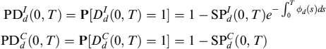
where ![]() and
and ![]() . It is worth noting that we included the effect of the time-dependent function ϕd,t within the idiosyncratic default event.
. It is worth noting that we included the effect of the time-dependent function ϕd,t within the idiosyncratic default event.
Let VColl(t) be the value of the portfolio of bonds used as collateral, formed as:
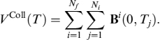
In a repo transaction or collateralized loan, the lender seeks to make the expected loss equal to zero over a given period from 0 to T. The expected loss (EL) is equal to the expected exposure at default (EAD) minus the value of the collateral, in the event of default of the counterparty i. The EAD is simply the amount lent (assuming no scheduled repayments between 0 and T), so that:
It is straightforward to check that:
E[EAD|Dd(0, T) = 1] = EAD
If the amount lent is L then E[EAD] = L. Then we have:

where DColl(0, T) is the indicator function equal to 1 if at least one issuer of the bonds in the collateral portfolio has gone bankrupt by time T, and LGD is the loss generated by the default events. The equation can be rewritten as:

We split this equation into two parts. In this case it is also clear that:
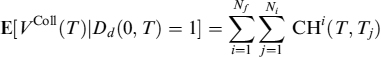
since VColl(T) is the value of the portfolio at time T given that no default event has occurred. CHi(T, Tj) is the expected price at time T of a coupon bond issued by i expiring at time Tj > T, defined as in (8.158). We assume that an issuer does not have more than one bond expiring on a specific date. The second part is:
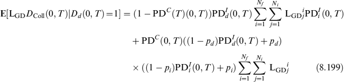
The first part of the right-hand side considers the expected value of the loss on bonds in the event of the counterparty's default, given that the common default event is not triggered (the amount is weighted by the probability that the common event does not occur: 1 − PDC(T)(0, T)); the second part is the expected value of the loss when the counterparty goes bankrupt and a common default event occurs (the amount is weighted by the probability that the common event occurs: PDC(T)(0, T)).
Making the simplifying assumption that ![]() with
with ![]() equal to the notional amount in the portfolio is a constant percentage of the par value of the bond, then we can rewrite the equation for the expected loss on the repo as:
equal to the notional amount in the portfolio is a constant percentage of the par value of the bond, then we can rewrite the equation for the expected loss on the repo as:
By the same token we can also compute the maximum loss at a defined confidence level, say 99%. This is quite easy to obtain since we already showed how to compute the minimum level of a portfolio of bonds at a given quantile by a Δ − Γ approximation; let the minimum value at the 99% c.l. of the portfolio at time T be:
![]()
where v is the quantile calculated as shown in Section 8.5. Then the maximum loss is:
ML(T) = L − v + E[LGD Dcoll(0, T)|Dd(0, T) = 1]
The fair haircut to apply to the value of the portfolio of bonds at the inception of the repo or collateralized loans is the level that makes the EL or the ML zero, depending on whether the bank wants to be more or less conservative. If the bank chooses to make the EL zero, considering that the amount lent at time 0 is equal to the value of the portfolio V(t) minus the haircut, L =(1 − H)V(0), the level of H is chosen so that:
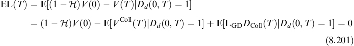
If the bank wants to compute the haircut based on the minimum level of the portfolio of bonds, then:

where vDI is the quantile of the portfolio including default events as defined in Section 8.5.5.
It is interesting to measure the degree to which wrong-way risk impacts on the haircut. To this end we have to apply the formulae above assuming that no correlation exists between the counterparty and the issuer of the bond. In our setup this means that the parameter p is equal to zero for each debtor, or that the probability of a common credit event PDC = 0. Nonetheless, we still want the total PD of each debtor to be the same as that produced by the combined effect of both the idiosyncratic and common factors. This means that in the absence of wrong-way risk it is
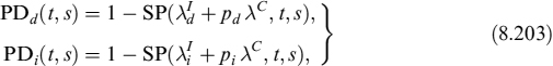
where SP is the zero-coupon bond in equation (8.27). Equation (8.199) modifies as follows:
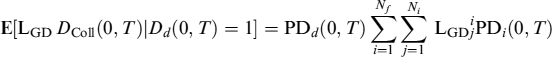
The haircut is then computed as indicated in equations (8.201) and (8.202).
Example 8.6.1. We consider a portfolio of Italian bonds, used as collateral for two firms (UCG, ISP), on June 6, 2012. The specifics for the ITA bonds (collateral) and the UCG, ISP bonds (portfolios) are given in Table 8.20.
Assume that the bank has to lend money to another bank and that it accepts as collateral Treasury bonds. Let the counteparty borrowing money be either Intesa Sanpaolo (ISP), an Italian bank, or Unicredit Group (UCG), a European international bank. Moreover, we assume that the collateral comprises bonds issued by the Italian Treasury (ITA). The collateral is posted at the start of the contact and is not updated until maturity.
The interest rate process follows a CIR++ model and the parameters are those estimated in Example 8.5.1. To estimate the parameters of the default intensities of the two possible counterparties and of the Italian Treasury, we consider the prices of the bonds issued, respectively, by ITA, UCG and ISP, with the specifics in Table 8.20, over the period from 12/31/2010 to 6/4/2012; we set the reference date as 4/6/2012. For each bond, we take into account the time series of prices from the issue date to the reference date. We calibrate the values of the parameters with the term structure of bond prices using the Kálmán filter technique, obtaining the results in Table 8.21.
In Figure 8.15, we plot the intensity of default λt for each issuer ITA, UCG and ISP, over the period 12/31/2010 to 6/4/2012.
In Tables 8.22–8.24, we show the fair haircut (based on the EL and the ML) that the bank should apply for a repo or a loan secured with UCG or ISP maturing, respectively, in s = 3M, 6M and 1Y, for the three cases in which the collateral is a portfolio of the five Italian bonds above, the Italian bond maturing on 01/05/2017, and the other Italian bond maturing on 01/03/2022. We show the results both when we include wrong-way risk (WWR) and when we exclude it.
Haircuts are typically revised periodically to get the credit risk of the repo or collateralized loan back to as close to zero as possible. If the life of the contract is the period [0, T], divided into n subperiods of length [Ti−1, Ti], for 0 ≥ i ≤ n and T0 = 0, then the haircut has to be calculated every time according to the methodology we have sketched above, with the default risk referring to the subperiod [Ti−1, Ti], instead of the total period [0, Ti]. So, at the inception of the contract, the haircut is obtained, according to the expected or maximum loss, by solving the equations:
Table 8.20. Specifics for the bonds issued by the Italian Treasury, Unicredit and Intesa Sanpaolo bank
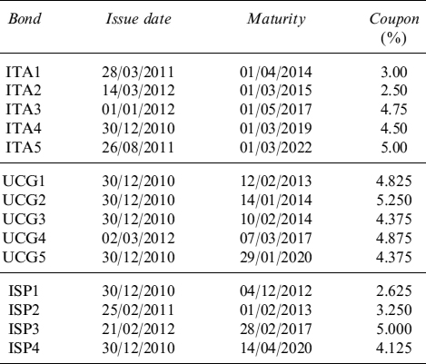
Table 8.21. Values of the parameters of the CIR model for the intensity of default process for the issuers Italy, Unicredit and Intesa Sanpaolo Bank, obtained with the Kálmán filtering technique
| Parameter | Value |
| κ | 0.0276 |
| θC | 4.517% |
| θITA | 9.075% |
| θUCG | 9.505% |
| θISP | 9.505% |
| σC | 5.679% |
| PITA | 0.8394 |
| PUCG | 0.7984 |
| PISP | 0.8175 |

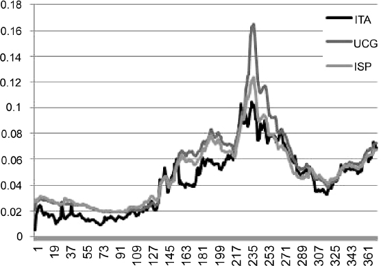
Figure 8.15. The value of the default intensity as a function of time, for the three issuers Italy, Unicredit and Intesa Sanpaolo bank, obtained from the Kálmán filter technique described
Table 8.22. Haircuts based on the EL and ML. The collateral is the portfolio of Italian bonds
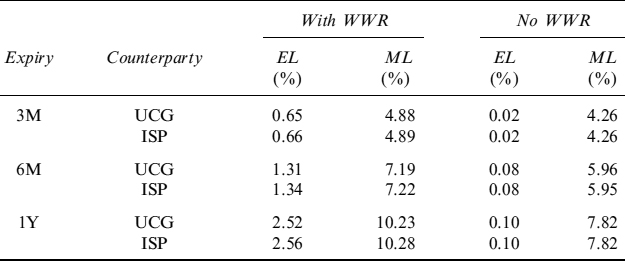
and
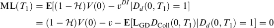
Then in T1 the haircut is revised using new-market data and PD data by computing EL(T2) or ML(T2), and so on until the end of the contract.
Table 8.23. Haircuts based on the EL and ML. The collateral is the bond maturing on 01/05/2017
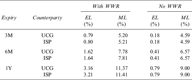
Table 8.24. Haircuts based on the EL and ML. The collateral is the bond maturing on 01/03/2022
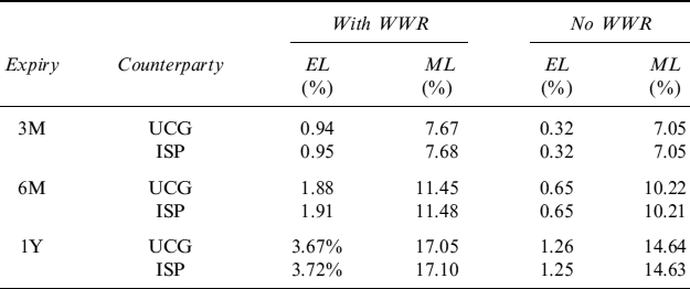
8.7 ADJUSTMENTS TO THE VALUE OF ILLIQUID BONDS
Banks do not only have liquid bonds on their balance sheet for liquidity management purposes. Often some assets are liquid and actively traded in the market in the first part of their life, but afterwards the trading activity becomes scant and they no longer can be considered liquid. In these cases the bank will likely hold the assets until their maturity, but it is always possible that they can be sold to extract liquidity, although the trading process takes much longer to complete (maybe weeks or even months).
The problem with illiquid assets is twofold:
- A fair value has to be attached to them which cannot directly be retrieved from the market, for the very fact that they are not actively traded. The fair value does not consider any difficulty in trading the bond such that it only refers to the case when it is perfectly liquid. So, attributing a fair value to an illiquid asset can only be carried out by disregarding any liquidity effects and by pretending that the asset is liquid.
- An adjustment should be added to the fair value to reflect the actual capacity of the asset to generate liquidity, in terms of the amount and time needed.
Limiting our analysis to bonds, the fair value can easily be computed if other liquid bonds issued by the same debtor are actively traded in the market. In fact, based on them, it is possible to estimate the parameters of a model of the credit risk run by the issuer, such as the composite intensity framework we have used above to predict the LGC of a bond portfolio. Applying the credit model to illiquid bonds jointly with an interest rate model that has been also properly calibrated, allows computing the fair value with a relatively good degree of accuracy and reliability.
The liquidity adjustment to the fair value requires more care. The adjustment, as will be clear from what follows, is not an objective correction to the value, meaningful for any holder. It depends on subjective factors, such as the funding spread of the holder, the amount of the bond held on the balance sheet and, finally, the probability of selling the bond before its expiry. On the other hand, objective factors also play a role in defining the adjustment to the fair value: the trading activity of the bond, identified by the number of times it trades in the market in a given period and average amount. The combination of these two types of factors determine the liquidity adjustment to the fair value of the bond that refers to the specific holder—not a quantity that can be applied “objectively” to the bond.
The model we present hinges on two considerations:
- A long position in an illiquid bond that cannot be sold immediately, but only over a certain period that depends on its trading activity, can be made comparable, in terms of generation liquidity, with a position in a liquid bond that can be immediately sold, if the bank borrows the amount that it would receive if the position were in the liquid bond, and then repay the loan as it receives the money from the selling of the illiquid bond during the period that is required to complete the trade. This strategy has clearly a cost that depends on the funding spread that the bank has to pay for the period needed to fully dismantle the position. We name the correction to the fair value of the bond due to this cost as liquid equivalent adjustment (LEA).
- During the time required to completely sell the amount of the bond, the price of the bond can move up and down. The bank is interested in forecasting adverse movements and then computing the maximum loss (at a certain confidence level) it could suffer for not being able to sell immediately the amount held. The loss is given by the difference between the value of the position in the bond at the time the bank decides to sell it, and the minimum value of the position during the period required to completely sell it. We term the correction to the fair value of the bond due to this loss as price volatility adjustment (PVA).
Both adjustments have to take into account the fact that the costs (for LEA) and the loss (for PVA) are borne by the bank only if it decides to sell the position in the future. So they have to be weighted by a selling probability that will then be included in the model. The sum of the two adjustments is the liquidity adjustment (LA) to the fair value. The adjusted price is the liquidity that can be expected to be extracted from the position in an illiquid bond.
Remark 8.7.1. The model we present produces the LA assuming that the bank wants to sell the entire amount held when it decides to do so. In reality, it is possible to consider cases when only partial liquidation of the position is planned as well. In this case the adjustment has to be computed with respect to this amount, smaller than the total amount on the balance sheet, so that it will be different. It is then possible to calculate a range of LAs depending on the different fractions of the total amount that have to be sold.
8.7.1 Liquid equivalent adjustment
Let us focus on the LEA component of the LA. Assume that at time t we wish to compute the liquidity adjustment for a bond maturing at T. Let B(t, T) be the fair value at time t; the expected price of the bond at a future date s is CH(t, s, T). We work within the framework described in Section 8.5 to evaluate the bond and we use the same notation. The amount held by the bank on its balance sheet is N.
The bond is not actively traded in the market: we first need to model the trading activity. Let the average traded amount of the notional of the bond be ![]() , and let the trades occur with a trading intensity at time t equal to λT(t). Trading intensity indicates how many trades occur in a short period dt; the inverse of the intensity 1/λT(t) gives the expected time elapsing before a new trade occurs.
, and let the trades occur with a trading intensity at time t equal to λT(t). Trading intensity indicates how many trades occur in a short period dt; the inverse of the intensity 1/λT(t) gives the expected time elapsing before a new trade occurs.
For example, assume that ![]() and that λT(t) = 365. This means that the bank can expect to trade 1,000,000 notional every λT(t) = 1/365 of a year, or every day. If λT(t) = 182, then 1,000,000 notional is expected to trade approximately every 2 days.
and that λT(t) = 365. This means that the bank can expect to trade 1,000,000 notional every λT(t) = 1/365 of a year, or every day. If λT(t) = 182, then 1,000,000 notional is expected to trade approximately every 2 days.
Trading intensity is modelled as a deterministic function of the kind
where ![]() is the trade intensity at t = 0, λ−T is the long-term average trading intensity. Usually, bonds start with good trading activity after their issuance, then the number of deals gradually fade away during the life and, finally, the market becomes scant as the maturity approaches. This pattern can be modelled by setting a high trading intensity just after issuance of the bond (e.g., λT(0) ≥ 365 for trades occurring at least once a day), and a low long-term average intensity (e.g., λ−T ≤ 25 for trades occurring less than once a fortnight). The speed at which trading activity is pushed towards the long-term average is commanded by the parameter κT.
is the trade intensity at t = 0, λ−T is the long-term average trading intensity. Usually, bonds start with good trading activity after their issuance, then the number of deals gradually fade away during the life and, finally, the market becomes scant as the maturity approaches. This pattern can be modelled by setting a high trading intensity just after issuance of the bond (e.g., λT(0) ≥ 365 for trades occurring at least once a day), and a low long-term average intensity (e.g., λ−T ≤ 25 for trades occurring less than once a fortnight). The speed at which trading activity is pushed towards the long-term average is commanded by the parameter κT.
The probability that the bank decides to sell the bond can be modelled by an intensity process as well: in this case we want to make the probability dependent on the default probability of the bank, since when the latter increases there is a higher probability that the bank may wish to sell less liquid assets to avoid paying high credit spreads over the risk-free rate. Thus, the selling intensity is:
where f(t) is a deterministic function and ![]() is the bank's default intensity, which is in turn a composite intensity as in Section 8.5. This formulation will also allow wrong-way risk to be considered (i.e., a higher probability to sell the bond when its value is lower due to the higher default probabilities of the issuer). Using the property of the CIR process, we write the selling intensity as
is the bank's default intensity, which is in turn a composite intensity as in Section 8.5. This formulation will also allow wrong-way risk to be considered (i.e., a higher probability to sell the bond when its value is lower due to the higher default probabilities of the issuer). Using the property of the CIR process, we write the selling intensity as
so that μ(t) is a process. Here, for the function f(t), we take a deterministic function of the type
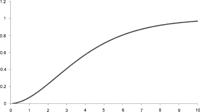
Figure 8.16. The probability of selling as a function of time (in years) for the parameters given in Table 8.25
so that the integral is

It is also easy to check that when the PD of the bank (i.e., the holder of the bond) increases, selling intensity increases as well by a factor α. The probability of selling the bond between two times s and T is
where PNS(t0, t) is the probability that the bond is not sold within [t0, t], which is available in a closed-form formula in our setting:
where ![]() is given in (8.27). In Figure 8.16 we show the probability of selling as a function of time for the selling parameters in Table 8.25.
is given in (8.27). In Figure 8.16 we show the probability of selling as a function of time for the selling parameters in Table 8.25.
Table 8.25. The selling parameters used for Figure 8.16
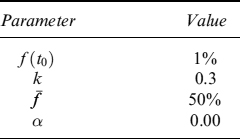
Given this setting, at time t the bank has to operate an expected number of ![]() transactions to sell the entire position it holds; with selling intensity equal to λT(t), the average time Tl(t) to close out the position is:
transactions to sell the entire position it holds; with selling intensity equal to λT(t), the average time Tl(t) to close out the position is:
If the bank wants to have the money it would receive if the bond were liquid immediately, it has it to borrow an amount of money equal to N × B(t, T). The borrowed amount is gradually paid back as the selling process completes; meanwhile the bank pays interest on the outstanding debt it has. The total interest rate the bank pays is composed of the risk-free rate plus a funding (credit) spread; on the other hand, the bank still earns the yield on the part of the position in the bond that has not yet been sold (which equals the outstanding debt). For equilibrium the yield on the bond's position should match the risk-free rate so we assume that on an expectation basis the net cost paid by the bank is the funding spread.
Over the period [t, t + Tl(t)] the annualized funding spread required of the bank is:15
where LGD is the loss given default percentage (e.g., LGD = 60%) and PDB is the default probability of the bank.
The LEA is the present value of the expected costs paid by the bank in case it decides to sell the bond, weighted by the probability of selling:
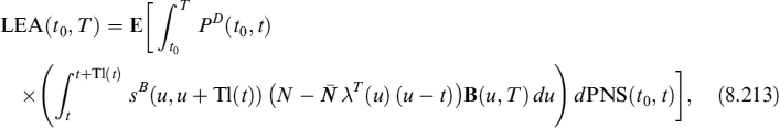
where sB(u, u + Tl(t)) is the stochastic spread rate applied for the period [u, u + Tl(t)] and PD(t, u) is the discount factor for the short-rate rt over the period [t, u].
Over the period [t, t + Tl(t)], we approximate the spread and the price of the bond with its value in t. This is a good numeric approximation, since the liquidation time ranges from one day to a few months, and the integral over du can be performed numerically by using a few integration points. The integral in equation (8.213) is then approximated as
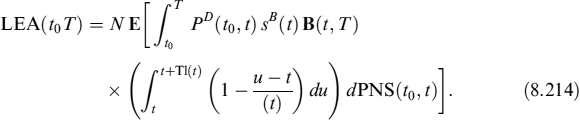
where sB(t) = sB(t, t + Tl(t)). The integration over du is

The liquidity adjustment in equation (8.214) is then

Numerical evaluation
To compute the value of the LEA, we consider a set of n dates Ti at which the selling of the bond might occur. We define the liquidation time at Ti with Tli = Tl(Ti). The liquidity adjustment in equation (8.216) reads
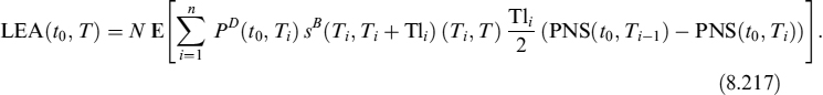
Taking the expression for the spread as in equation (8.212), the expression for LEA(t0, T) reads
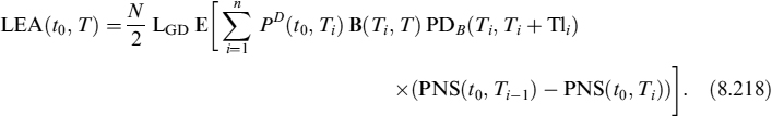
Defining the function
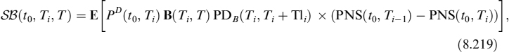
the expression for the LEA(t0, T) is
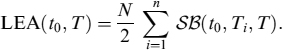
The expression for SB(t0, Ti, T) can be cast in a closed form (details are given in Appendix 8.A).
8.7.2 Price volatility adjustment
The second component of LA is the adjustment due to the losses the bank can incur during the liquidation period, since the bond price can divert from the level at the time the selling process starts. We define this as Price Volatility Adjustment (PVA). Consider a bond of maturity T. At time t0, let the expected (future) in t be CH(t0, t, T); the value of the portfolio can also drop, at time t, to Vp(t0, t) for a certain confidence level p.
To compute PVA, we cannot apply the procedure in Section 8.7.1 to separate the expected value of the product from the probability of selling and the quantile. In the present case, we need to compute the expectation value in the forward risk-adjusted measure with respect to the short rate r and to the default intensity processes. Let us define PVA as
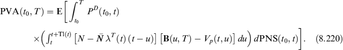
Similarly to the case of LEA(t0, T), we assume that the selling of the bond can happen only at specific dates Ti. The expression in equation (8.220) reads
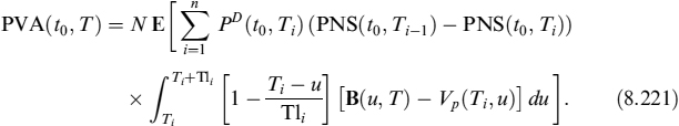
To evaluate PVA(t0, T) numerically, we first consider the expectation value appearing in equation (8.221). We take this expectation value in the forward measure ETi, Ti, where the first index refers to the Ti-forward measure with respect to rt, and the second index refers to the Ti-forward measure with respect to λ. We obtain
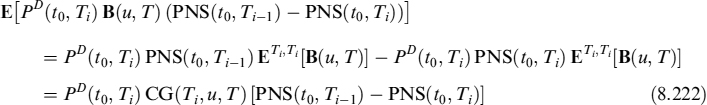
where CG(t, s, T) indicates the forward at time t for a bond with expiry s and maturity T, in the measure described above. Explicitly, it is
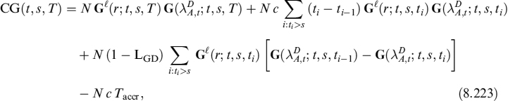
where ![]() is the default intensity of the bond's issuer, which follows the usual composite CIR++ dynamics, and the accrued time is
is the default intensity of the bond's issuer, which follows the usual composite CIR++ dynamics, and the accrued time is
Taccr = s − max(tl : tl ≤ s),
and ![]() is given by
is given by
![]()
where ![]() is the bond-specific parameter to capture liquidity specialness and G is the zero-coupon bond forward price given in equation (8.31). The expression in equation (8.221) reads
is the bond-specific parameter to capture liquidity specialness and G is the zero-coupon bond forward price given in equation (8.31). The expression in equation (8.221) reads
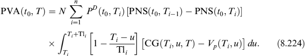
To compute the quantile, we refer to the procedure outlined in Section (8.5.5), with the following modification. First, all futures appearing in the formulae are replaced by the corresponding expressions for the forwards in equation (8.223). Second, the mean and the covariance matrix of the short rate and of the default intensities are taken in the forward risk-adjusted measure. Following the result in Appendix 8.A, the mean is
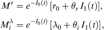
while the covariance matrix is
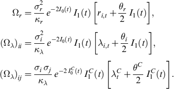
We defined the integrals
while ![]() and
and ![]() are the same as the CIR parameters for the common intensity of the default process λC(t) used. Explicit formulae for the integrals are given in Appendix 8.A.
are the same as the CIR parameters for the common intensity of the default process λC(t) used. Explicit formulae for the integrals are given in Appendix 8.A.
Numerical evaluation of the integral in equation (8.224)
In computing the value of PVA(t0, T), we cannot approximate the function CG(Ti, u, T) − Vp(Ti, u) appearing in equation (8.224) to its value in Ti, because at the selling time the quantile equals the value of the bond and the expected loss is zero. In order to include the expected loss in the numerical computation of the integral over du, we use the following procedure
- we divide the period [Ti, Tli] into m fractions;
- we introduce the time step
- we introduce the integration points
- At the integration point u = tk, we substitute
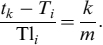
The integral over du in equation (8.224) is then approximated by
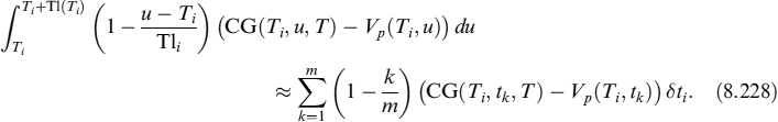
With this approximation, the expression in equation (8.224) reads
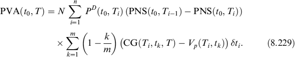
Total liquidity adjustment for the bond is then:
Example 8.7.1. In the following example, we consider a bank with characteristics similar to Unicredit (UCG, see above) wants to value a bond issued by Intesa Sanpaolo (ISP) with the specifics in Table 8.26. In Table 8.27, we show the CIR parameters used to describe the default intensity of UCG and ISP. We assume that the bond can be sold only at specific dates Ti, with constant semiannual intervals Ti − Ti−1 = 6M. In Table 8.29, we show results for the term structure of the probability of selling at each Ti the LEA, the liquidation time in days, the expected loss over [Ti, Ti + Tli] and the values of PVA and total liquidity adjustment LA = LEA + PVA, when the parameters in Table 8.28 are used.
Table 8.26. Specifics of the ISP bond for which the liquidity adjustment is computed
| Parameter | Value |
| Maturity | 14/4/2020 |
| Coupon rate | 4.1250% |
| Market price | 87.5480 |
Table 8.27. Parameter values of the model for the intensity of default process for UCG and ISP
| Parameter | Value |
| λC | 6.06% |
| λUCG | 3.51% |
| λISP | 3.99% |
| κ | 0.0276 |
| θC | 4.517% |
| θUCG | 9.505% |
| θISP | 9.505% |
| σC | 5.679% |
| PUCG | 0.7984 |
| PISP | 0.8175 |
Table 8.28. Parameters used for the results in Table 8.29
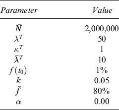
Table 8.29. The term structure of liquid equivalent adjustment (LEA), liquid volatility adjustment (PVA) and total liquidity adjustment LA = LEA + PVA, for the parameters used in Table 8.28
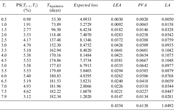
Example 8.7.2. Keeping Example 8.7.1 in mind, we consider the case in which the liquidation time is much shorter when the bond is sold in the first years. Table 8.30 gives the entire set of parameters used. λT = 730 indicates that the bond trades in the market on average three times a day, in an amount of ![]() . The results are in Table 8.31.
. The results are in Table 8.31.
Example 8.7.3. Keeping Example 8.7.1 in mind once again, we consider the case in which the parameter of mean reversion governing the selling probability of the bond is higher. This means that before expiry of the bond, there will be more chances that the bond will be sold by UGC. Table 8.32 gives the parameters and the results are shown in Table 8.33.
Table 8.30. Parameters used for the results in Table 8.31
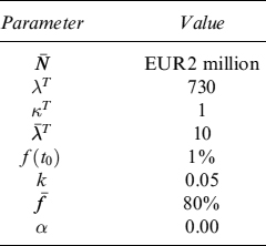
Table 8.31. The term structure of the liquid equivalent adjustment (LEA), the price volatility adjustment (PVA), and the total liquidity adjustment LA = LEA + PVA, for the parameters used in Table 8.33

Example 8.7.4. Keeping Example 8.7.1 in mind yet again, we show the impact of parameter α, which regulates the impact of the stochastic component of the probability of selling depending on the probability of default of the bank (UCG in this case). The results are shown in Figure 8.17 for the parameters in Table 8.34.
Conditioned selling probability
In this section we will show how the results presented in the previous examples modify when we assume the bank will definitely sell the bond within the maturity T. To consider this case, we introduce the probability of selling conditional to the selling of the bond before expiry. We impose that the probability of not having sold the bond within T is given the value of zero or, equivalently, the probability of selling before T the value of one. To achieve this, we divide the probability of selling presented in equation (8.209) by the probability of selling the bond after T, so that it becomes a conditional probability:
Table 8.32. Parameters used for the results in Table 8.33
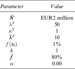
Table 8.33. The term structure of liquid equivalent adjustment (LEA), price volatility adjustment (PVA) and total liquidity adjustment LA = LEA + PVA, for the parameters used in Table 8.32
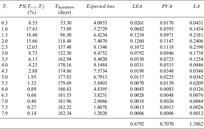
The conditional probability of selling thus defined satisfies
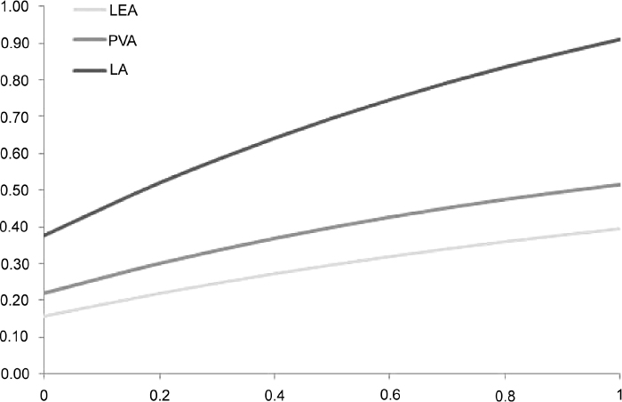
Figure 8.17. LA, LEA and PVA as a function of parameter α (x-axis). The other parameters are given in Table 8.34
Table 8.34. The selling parameters used for Figure 8.17
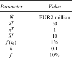
Example 8.7.5. In this example we keep the results presented in Examples 8.7.1, 8.7.2 and 8.7.3 in mind, where UCG computes the liquidity adjustment on an ISP bond using the specifics in Table 8.26.
When the conditional probability of selling PS′(t0, t) is used instead of PS(t0, t), the results obtained in the examples above modify as follows. In Table 8.35, we show the results when the trading and selling parameters are the same as in Table 8.28. In Table 8.36, we show the results when the trading and selling parameters are the same as in Table 8.30, where the initial value of trading intensity is higher than in the first example. Finally, in Table 8.37, we show the results when the trading intensity and the selling parameters are as given in Table 8.32. In Figure 8.17, LA, ELA and PVA are plotted as a function of parameter α.
Table 8.35. The term structure of liquid equivalent adjustment (LEA), price volatility adjustment (PVA) and total liquidity adjustment LA = LEA + PVA, for the parameters used in Table 8.28
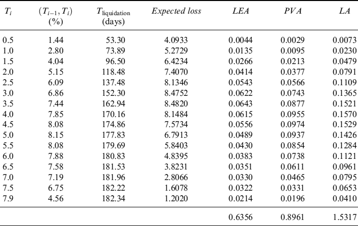
Table 8.36. The term structure of liquid equivalent adjustment (LEA), price volatility adjustment (PVA) and total liquidity adjustment LA = LEA + PVA, for the parameters used in Table 8.30
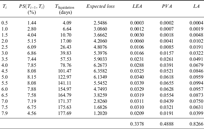
Table 8.37. The term structure of liquid equivalent adjustment (LEA), liquid volatility adjustment (PVA) and total liquidity adjustment LA = LEA + PVA, for the parameters used in Table 8.32
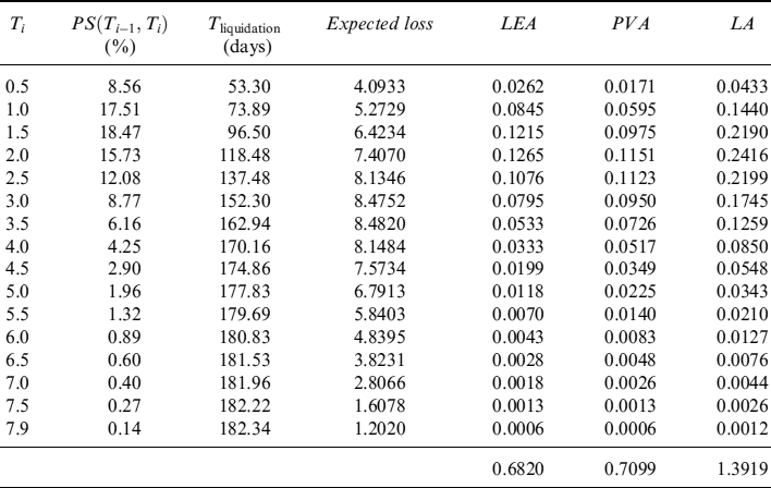
APPENDIX 8.A EXPECTATION VALUE OF THE BOND WITH SELLING PROBABILITY AND SPREAD
In this section, we compute the expectation value in equation (8.219). We write this expression as
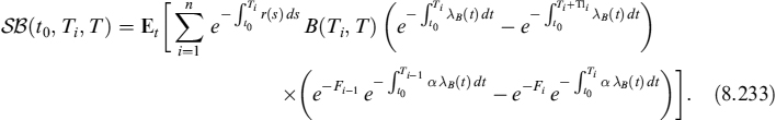
In equation (8.233), we explained the expressions for PD(t0, Ti) in terms of the stochastic short-rate r(t), and the expressions for PDB(Ti, Ti + Tli) and PNS(t0, Ti) in terms of default intensities. Moreover, B(Ti, T) is the expression for a defaultable coupon bond, see equation (8.157), before the expectation value is taken,
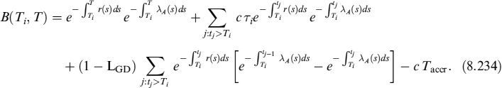
The quantity in equation (8.234) is the sum of four terms, so that SB(t0, Ti, T) in equation (8.233) can be split into four terms as well. For example, we show explicitly the computation involving the term
and the part in equation (8.233) containing this term reads
where we set the integral of the deterministic selling function Fi = F(t0, Ti). The expression in equation (8.235) is the sum of four distinct terms, coming from cross multiplication of the default probability times the probability of selling the asset over the period considered. For example, the first term in the sum in equation (8.235) is
![]()
We split processes λB and λA into an idiosyncratic and a common component and we arrange terms, thus obtaining
We take the expectation value in the tj-forward measure with respect to rt and ![]() , so that the expression above is
, so that the expression above is
we obtain
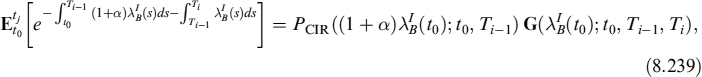
and
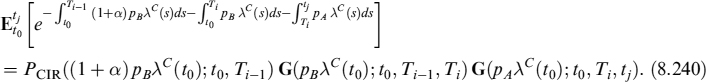
Summing up, the expectation value is
Computing all four expectation values in equation (8.235), and repeating the computation for all four terms in the expression for the coupon bond in equation (8.234) and rearranging, we finally obtain the expression for the bond with the probability of selling and the spread in equation (8.219) as
SB(t0, Ti, T) = PCIR(r; t0, Ti)F(Ti)B(t0, Ti, T),
where

and we define the coupon bond when the selling probability is included as
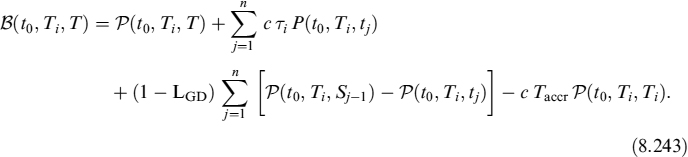
We now introduce for notational convenience the function
with, if tj > Ti + Tli,

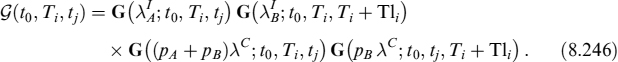
Eventually, LEA is written in the more readable form
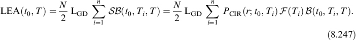
The forward risk-adjusted measure
In the T-forward measure, a CIR process reads
Brownian motion in the T-forward measure is
![]()
and the mean reversion speed is
![]()
with the CIR factor
and ![]() .
.
Mean in the FRA measure
In the following, we indicate the mean value of rt in the T-forward measure with
Taking the expectation value of equation (8.248) in the T-forward measure, we find that E1(t) satisfies the differential equation
To solve for E1(t), we first compute a solution to the homogeneous part of the differential equation,
or
where r0 is the value at time t = 0 of the interest rate. To find a complete solution to equation (8.250), we use the method of the variation of constants. For this, we write
where the function r0(t) follows a differential equation which is obtained by plugging equation (8.253) into equation (8.250), giving
with the formal solution
Finally, a solution to the inhomogeneous equation (8.250) is given by the sum of the solution found by the methods of the variation of constants plus the homogeneous solution,
As a check, we impose a constant ![]() , obtaining
, obtaining
which is precisely the expression for the average value of rt in the risk-neutral measure.
For the CIR model, this expression can be cast in a closed-form formula, since
It can be shown that, in the limit σ → 0, the expression above reduces to κ t. We have
and
The complete expression for the mean of the CIR process in the T-forward measure is
Volatility in the FRA measure
Let us try to find the value of the quantity
Setting
Using Ito's lemma, the quantity r(t)2 follows the process
where in the last equality we used the expression in equation (8.248) for the CIR process in the T-forward measure. Taking the expectation value on both sides, we obtain
The solution to the homogeneous equation is
The solution to the inhomogeneous equation is the sum
where the function v(t) is fixed by using the method of the variation of constants. We find
with the formal solution
Setting
and
we find that the volatility is
However, the second term is unnecessary, since we find that

and
so 2I2(t) − I(1)2 = 0. The volatility in the T-forward measure is then
When σ → 0, and γ → κ, this equation reduces to the usual expression for the volatility in the risk-neutral measure,
1 We are in grateful to Luca Visinelli for discussions with one of the authors in the development phase of the models presented in this chapter. Moreover, he gave invaluable support in implementing and testing them in the examples shown below.
2 Some currencies such as the yen and the Swiss franc experienced negative levels of the interest rates for short expiries, typically up to one year.
3 The future price, as well as the forward price we show immediately below, should not be confused with the value of the contract. They are simply the price level making the value, respectively, of the the future or the forward contract equal to zero.
4 If we assume that the Libor and Euribor rates are not risk-free rates and we model them using a CIR model, then we can also price caps and floors on Libor or Euribor fixings. In the current market environment the assumption that Libor/Euribor fixings are risk-free rates is believed to be too strong and the model will work poorly to price this type of contract. Anyway, the example we suggest of caps and floors on Eonia rates admittedly refers to unusual contracts traded in the market.
5 See also [59] on this point.
6 The model was introduced and analysed in [34], to which we refer the reader for more details.
7 These types of processes are studied in [59] and [82]. See also [33] for an application to credit derivatives pricing.
8 For the default intensity process we further assume that the market risk parameter is equal to zero, so that risk-neutral and real measure drifts are the same.
9 Under the assumption that the the market risk parameter is zero, the future price formula can also be used to calculate the expected price in the real measure, provided that we use a volatility parameter estimated from the historical time series and not implied from quoted caps, floors or swaptions.
10 See the ECB's guidelines on liquidity policy [17].
11 The model we present is based on [60]. We refer to it for technical details.
12 We are absolutely aware we are restricting the analysis to a limited number of banks with respect to all financial institutions operating worldwide.
13 At the time of this writing, the crisis is still not over.
14 This approximation was used by Duffie and Pan [60]. We ignore the double-counting of defaults that occurs with both common and idiosyncratic credit events. The approximation also undercounts defaults associated with multiple common credit events before time T. These two effects partially offset each other.
15 See Section 8.4.