Camera Exposure Value, EV, and Matching EV to LV

The primary photographic challenge, especially in landscape astrophotography, is to collect the right amount of light to produce a properly exposed image, regardless of the amount of light originating from the scene. Historically, a “properly exposed” image is one with an overall brightness that is 18 percent gray, or 18 percent of the way between black and white. When we view scenes with differing light values with our eyes, our vision system handles this light collection and conversion process automatically; for example, our irises dilate/contract and our retinas become more or less sensitive. In photography, however, this process is done by the photographer, and is accomplished by setting the exposure value (EV) of the camera to correspond to the light value (LV) of the scene, Chapter 10. The EV depends mathematically on the ISO, I, aperture, A, and shutter speed, T, according to the logarithmic relationship:

Several tables of camera EVs calculated for different ISO, aperture, and shutter speed combinations are shown in Figure 12.1. These results make it clear that there are many possible combinations of different exposure settings that result in the identical EV. To summarize, when we match the camera EV to the scene LV, we are assured of obtaining a correctly exposed image, i.e. one that is on average 18 percent gray, even if the subject scene is extremely dark or bright. The overall brightness of the resultant image will be the same.

Now, in practical terms, rarely, if ever, will you need (or want) to actually calculate your camera’s numerical EV, since your camera’s built-in light meter and analysis system does all the work for you. Instead, by taking a light meter reading of the scene of interest, you will be shown whether your current combination of ISO, aperture, and shutter speed is suitable to match the scene LV, or if it is too high or too low and you might wish to make adjustments. However, your understanding of: (a) the LV levels of typical landscape astrophotography scenes and (b) what combinations of ISO, aperture, and shutter speed are available to match them will be of enormous value in planning and avoiding a frustrating night of trial-and-error in the field while your subjects slowly slip below the horizon in front of your eyes!

By way of example, imagine that we want to create a nightscape image with the Milky Way on a moonless night, e.g. Figure 8.1. We know from Table 10.1 that scenes such as these typically have an LV in the range of approximately −8 to −5. Therefore, we know that in order to match this light value to obtain a properly exposed image, we should set our camera to a corresponding EV of approximately −5. If our camera’s EV setting is set to correspond to a much dimmer LV, for example −12, the resultant image will be too bright. This is because the camera is set to receive less light than it actually would receive, like walking around in daylight with dilated pupils. On the other hand, if the camera’s EV setting is too high, say −2, then the resultant image will be too dark. In this case, the camera requires more light than is available for a properly exposed image. From Figure 12.1, we see that we can choose any of the following combinations; all of which produce a camera EV equal to −5:

12.1 Tables of camera exposure values (EVs) for different combinations of ISO, aperture and shutter speed. Note that there are many different combinations of ISO, aperture, and shutter speed that result in the identical EV. For example, an EV of −5 (purple), or −8 (yellow) which would be appropriate to match the LV of a typical Milky Way nightscape, can be achieved with any of the different combinations shown. The multiple different ways of setting the camera to an EV of nine, which would be more appropriate for the LV of a sunset scene, are highlighted in gold.

• ISO = 100, f/4 for 8 minutes
• ISO=800, f/4 for 1 minute
• ISO=800, f/11 for 8 minutes
• ISO = 6400, f/4 for 8 seconds
• ISO=6400, f/11 for 1 minute
• ISO = 6400, f/2.8 for 4 seconds

Okay, so the identical EV can be achieved from different combinations of ISO, aperture, and shutter speed. By now, I’m sure you’re asking the obvious question – out of all these possible combinations, which one is the best? In other words, which is the single, best combination of settings that will result in a trophy image worthy of enlarging for framing? Note there are some significant differences—for example, exposure times that range from 4 seconds to 8 minutes. Are they really all the same? My answer is that the precise manner in which the EV of the camera is chosen to correspond to the LV of the scene is perhaps the most foundational technical skill in photography.

Matching Camera EV to Scene LV—The Firefly Analogy

If this all seems confusing, don’t despair. My favorite way to understand the process of matching the EV of the camera to the LV of the scene is with the help of an adaptation of an analogy originally created by Bryan Peterson. Imagine that the light given off by the scene every second may be represented by individual “light fireflies,” as illustrated in Figure 12.2. For brighter scenes, more fireflies are given off per second than dimmer scenes, equivalent to the higher lux for brighter scenes shown in Table 10.1.

The goal is to allow the requisite number of fireflies to enter the camera to achieve a correct exposure. This goal is achieved by adjusting the combination of ISO, aperture, and shutter speed to set the camera EV to match the LV of the scene, regardless of its actual value at any given time. In doing so, you ensure that the camera will receive the correct number of fireflies for a correct exposure, every time, regardless of how many of them are being emitted by the scene.

Let’s go through a practical example. Imagine that we have determined that the LV of our scene is nine. For this exercise, we will thus say that we have nine fireflies per second being emitted from the scene, Figure 12.3(a). In this example, you may consider each firefly to represent one LV of scene brightness. In order to create a properly exposed image, therefore, we must set our camera’s EV to receive nine fireflies. How shall we do this?

Consider each of the three camera exposure settings: ISO, aperture, and shutter speed, to represent three categories, or buckets, into which any of the fireflies may be placed. In order to set the camera EV to nine, we need to distribute the nine fireflies between each of the three buckets. One possibility might be to put four fireflies in the ISO bucket, one in the aperture bucket, and four in the shutter speed bucket, Figure 12.3(b, left). Alternatively, we may elect to put two fireflies in the ISO bucket, five in the aperture bucket, and two in the shutter speed bucket, Figure 12.3(b, middle). Finally, we may choose just one firefly in the ISO bucket, two in the aperture bucket, and the rest in the shutter speed bucket, Figure 12.3(b, right). In each case, the overall image will have the same exposure—nine; what will differ will be the attributes resulting from the effects of the different camera settings. Let’s now examine some of the differences that arise in our landscape astrophotography images as we make the selections.

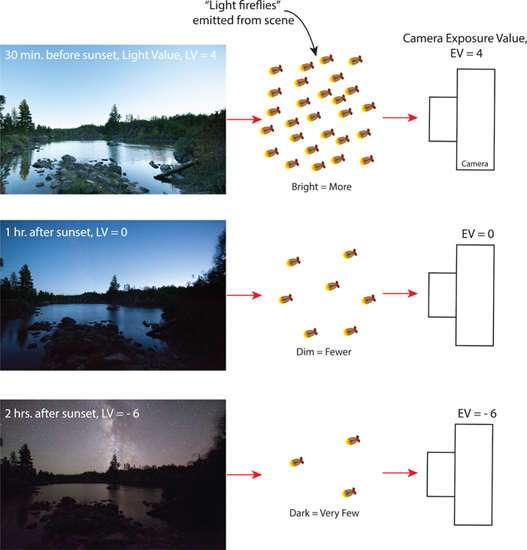
12.2 “Firefly” equivalents for three typical landscape astrophotography scenes. Brighter scenes have more fireflies given off per second compared to dimmer scenes. The scene LV and corresponding camera EV for a correct exposure are also shown.

12.3 Different ways of distributing the same number of fireflies, (a), between the categories of ISO, aperture, and shutter speed (b). This process ensures that we set the camera EV to match the scene LV, in this case, nine.

Aperture

In the vast majority of cases, you will want to set as low an aperture number, or f-stop, as is feasible. Notice I did not say as low as possible but feasible. There is an important difference. A low f-stop corresponds to an aperture that is physically large or wide open. So why not simply set the aperture to its minimum value, for example, f/2.8 or even f/1.4 to allow as much of the ambient light from the scene into our cameras as possible? You will recall from Chapter 11 that one reason is that an aperture set to its minimum value can allow lens imperfection effects, especially apparent in astrophotography. Also, images made at minimum aperture can appear noticeably softer, which, for example, can impact the appearance, or crispness, of the Milky Way.

An example of coma and how the choice of aperture affects its onset is shown in Figure 12.4. Note the clearly visible coma at minimum aperture—coma has the effect of distorting stars from round points of light into “flying seagulls.” Consequently, the best compromise between coma and a too-restricted aperture is generally to set your aperture to one to two stops above the minimum aperture of the lens: for a lens with a minimum aperture of f/2.8, that would be f/5.6; for one with a minimum aperture of f/4, that would be f/8.

12.4 Photographs of the constellation Orion at equivalent camera EV but different combinations of aperture and shutter speed, shown here in the left column. All four photographs were made with a 50 mm lens and an ISO setting of 6400.

Shutter Speed

The only real limitation on shutter speed, or exposure duration, in most landscape astrophotography images relates to undesirable effects of moving subjects. Distracting artifacts can manifest themselves as either unwanted streaking/trailing of stars or blurred foreground objects resulting from wind or other motion. In either case, keeping the shutter speed below a certain value will eliminate the appearance of movement. However, owing to restrictions on aperture such as coma, it may be necessary to keep the shutter open long enough to obtain a correct exposure. So, how long a shutter speed is too long?

For years, the practical “Rule of 400/500/600” has been the go-to guide for estimating the maximum exposure length that can be implemented without noticeable star trails. The idea is simple; just divide the number 400, 500, or 600 by the focal length of the lens (in millimeters) to obtain the maximum shutter speed (in seconds) that may be safely used. Using the number 400 gives the most conservative estimate and is my recommendation for those with higher-resolution cameras; using the number 600 may suffice for less critical audiences. Note: for users with crop sensor cameras, you will need to multiply the lens focal length by the crop factor (generally 1.5 or 1.6) to arrive at the correct focal length to use in the Rule of 400/500/600.

An example of the application of this rule is given in Figure 12.5, where six photographs of the constellation Orion are shown, all made with equivalent EV using a 50 mm lens but with different exposure times: 4, 8, 15, 30, 60, and 120 seconds. According to the Rule of 400/500/600, star streaking should be insignificant with exposure times less than 400/50 = 8 seconds, and likely to be starting to be noticeable after 600/50 = 12 seconds. Close inspection of the 15-second exposure shows barely discernible elongation of the stars; the 30-second image shows clearly visible distortion. Exposures of 60 and 120 seconds reveal more extensive streaking. The exposures made at 8 and 4 seconds show no signs of streaking, as predicted by the Rule of 400/500/600.

Finally, it is important to recognize that the relative motion of stars depends strongly on the compass direction you’re facing. For example, when facing north in the Northern Hemisphere, the apparent speeds of the stars is relatively less than the speeds of stars along the ecliptic, or when facing south. This is because the stars along the eclectic have to travel a greater distance (horizon–overhead–horizon) in the same amount of time as stars circling the celestial poles. This means that the maximum exposure time to avoid star trails can be longer when facing north than when facing south.

ISO

The ISO setting refers to the overall sensitivity of the camera sensor to light, and dictates how much light is needed to obtain a properly exposed image, or one that has an overall gray level of 18 percent. With reference to the firefly analogy, the camera EV is a measure of how many fireflies need to land on the sensor in order to make the image. Low ISO settings require enormous numbers of fireflies to produce a correctly exposed scene, whereas high ISO settings require far fewer fireflies. So why not simply set the ISO to the maximum possible setting?

Images made with a low ISO setting need lots of light. The results are images with very high resolution, in other words, images that can be enlarged without losing detail or revealing pixel noise or grain, Figure 12.6(a). In contrast, images made with high ISO generally suffer from distracting

12.5 Photographs of the constellation Orion made with equivalent EV but different exposure times: 4, 8, 15, 30, 60, and 120 seconds, from top to bottom. The onset of noticeably streaked stars becomes evident at around 15 seconds, and pronounced by 120 seconds. All six photographs were made with a 50 mm lens (minimum aperture of f/1.4). The region indicated by the white box is enlarged in the inset of each image to allow better visualization of the details of the images.

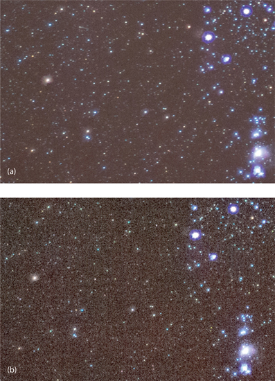
12.6 Photographs of stars taken with a 50 mm lens at equivalent camera EV but different ISO: (a) ISO = 3200; (b) ISO = 25600. Note the distinct graininess and color noise in the high ISO image (b) compared to the lower ISO image (a). Images made at even lower ISO have even better grain and color noise quality than (a).

graininess and often visible color noise, Figure 12.6(b). Why is this the case? Think of it as if you were making a painting made up of individual dots of paint. With high ISO images, you’re only allowed to use, say, 1,000 individual drops of paint to make up your painting, and so you have to use a fairly coarse brush. With a low ISO image, you would need 1,000,000,000 drops of paint and thus you are able to use an exceeding fine brush capable of exquisite detail. Herein lies the origin of the higher inherent quality of low ISO images, and their ability to be enlarged significantly without a loss of detail. Finally, images made at higher ISO settings exhibit less dynamic range and less color contrast, and have less capability for significant adjustments during post-processing.

Selecting ISO, Aperture, and Shutter Speed for Optimum Image Quality

It’s time to synthesize this knowledge into a cohesive strategy for producing the best possible landscape astrophotography image given the local conditions. Here are the key points so far:

• Matching camera EV to scene LV is the priority for a correctly exposed image
• Low ISO is better than high ISO, to minimize graininess and color noise
• The shorter the shutter speed the better, to minimize star trailing and foreground blur
• Best aperture is two stops above the minimum, to produce distortion-free images

We are now prepared to see how this knowledge is applied in the field.

Since we know what settings produce the highest quality images, why not just set the ISO to its lowest value, say, ISO = 100, set the aperture two stops above the minimum, say f/5.6 for a lens with a minimum aperture of f/2.8, and the shutter speed of the longest value needed to avoid star trailing, say 30 seconds for a 20 mm lens? With reference to the EV table in Figure 16.2, these settings result in a camera EV of EV = 0. Unfortunately, a great many landscape astrophotography scenes have much, much dimmer LVs, such as LV = −6 for scenes involving the Milky Way on moonless nights. This is a very significant difference; a camera set to an EV of 0 will unacceptably underexpose such a scene and will not work.

Consequently, we enter the arena of intentional trade-offs in camera settings. Suppose we bump up the ISO… how far can we go before the graininess is noticeable? How about the aperture… can we open it up more without terrible effects? And so on. Let’s go through an example to demonstrate the logic behind these tradeoffs. Once you have experienced this process a few times under night-sky conditions, you will develop your own set of references to refine and return to time after time. Remember, the goal is to maximize the time in the field acquiring images and minimizing the amount of time adjusting the exposure settings!

Four images were made for this optimization exercise, as shown in Figure 12.7. They were all produced using a 24 mm lens and a variety of exposure settings. The subject was the constellation Orion during a clear, moonless night. I wanted to compare three ISO settings: 1600, 3200, and 6400. I knew that an ISO higher than 6400 would just be too noisy for my liking and anything below 1600 was likely to result in an image that was so badly underexposed to be beyond salvaging. Then, I wanted to try two different apertures: f/2.8 and f/4. The minimum aperture for this lens was 2.8, so I knew there would be significant coma at the 2.8 aperture. The f/4 aperture, which was one stop above the minimum aperture would be better; I just wasn’t sure an aperture of f/5.6 would allow in enough light in a short enough time to avoid streaking of the stars. Finally, in order to set the exposure time, I turned to the Rule of 400/500/600 and calculated that as long as I kept the exposure time less than around 17–25 seconds with the 24 mm lens there shouldn’t be appreciable streaking of the stars. The settings of each of the four images is provided in Figure 12.7, along with the firefly analogy showing how the same overall number of fireflies are distributed amongst the three categories of ISO, aperture, and shutter speed.

Upon close examination of the images in Figure 12.7, as shown in the enlarged regions in the middle row, several trends are immediately apparent. Both exposures taken with a shutter speed of 30 seconds show an unacceptable level of streaking, which is consistent with the prediction of the Rule of 400/500/600 that any shutter speed greater than 17–25 seconds would show streaking.

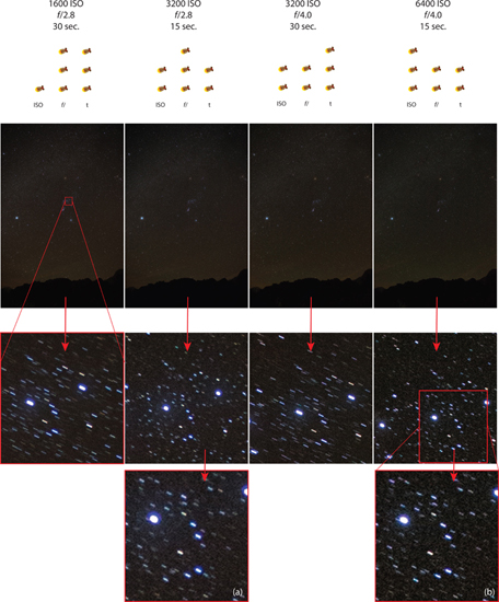
12.7 Example of the four images made during the optimization exercise described in the text. Also shown along the top is the manner in which the same total number of “fireflies” were distributed between the various exposure settings.

Of the remaining two images taken at 15 seconds, one with ISO = 3200 and the other at ISO = 6400, the 6400 image appears slightly crisper, albeit with a small increase in noise visible at this extreme magnification. However, the 6400 image was also made with an aperture of f/4, which we saw previously would result in less coma at the image periphery. Thus, my conclusion was that the optimum settings for this image would be ISO = 6400, f/4 for 15 seconds. Returning to the EV tables in Figure 12.1, we see that these settings produce a camera EV = −6, a result exactly suited to the LV of the dark sky conditions we are capturing.

To emphasize the significance of this outcome, recall that all four images in Figure 12.7 were collected at the same camera EV, yet only one of them produced “the best” image quality. It is very well worth your time studying this process and practicing a few of your own optimization experiments to really understand the tradeoffs.

A final example of how your choice of exposure settings can affect the resultant image appearance is shown in Figure 12.8 for the case of the Aurora Borealis. The overall exposure of both images in Figure 12.8 was adjusted through post-processing to result in the same EV in the final image. Changing the shutter speed from 30 seconds to 2 seconds dramatically increases the definition and structure seen in the auroral curtains. This is the result of the relatively rapid motion of the aurora. A 30-second exposure causes the individual structures to blur together, but a 2-second exposure maintains their definition.

Expose to the Right (ETTR)

The preceding example demonstrates a somewhat counterintuitive result that has become widely accepted in landscape astrophotography, namely, that higher ISO settings of 6400 or even 12,800 are preferable in many cases. One might imagine that the goal would always be to keep the ISO set to a low value and avoid the seemingly noisy higher ISO at all costs. Why is this? There are at least two reasons – the first relating to the ability to minimize star streaking by keeping the exposure time relatively short, as we saw in Figure 12.8. The second reason is that the downside of the minor degree of noise introduced at higher ISO levels is less than the amount of noise that would be seen by underexposing the image and then raising the exposure of the image in postprocessing, illustrated in Figure 12.9. The reason for this is that slightly overexposed images have far more tonal values to work with than underexposed images. This result has led to the conclusion that it is best to expose to the right (ETTR), a reference to the typical shape of the image histogram when exposed at higher ISOs at constant aperture and shutter speed than lower ISOs.

On many occasions, I have found myself at the start of a long night of shooting with an underexposed initial image, faced with tough decisions regarding which camera settings to change and by how much. Only by spending some time understanding these tradeoffs, gaining experience in making these changes, and then studying their actual impact does one really become proficient. As you progress, you may wish to note down a few initial settings for whatever scene LV you expect to encounter, and then use these as a starting point in the field. As we will see in Chapter 20, there are so many other things that can go wrong in the field that fiddling with exposure settings is the last way you will want to spend your time!

12.8 Comparison of exposure time on the appearance of the Aurora Borealis. Both images were made with an ISO setting of 6400 and an aperture of f/2.8. The image in (a) was made with a 2-second shutter spend and (b) a 30-second shutter speed. Both images were then adjusted using procedures described in Chapter 21 to have the identical final image brightness. The image made with the shorter time, (a), has much more clearly defined pillars and edges within the aurora than the image made with the longer time, (b).

12.9 The three images at the top were all collected with the same aperture and shutter speed but different ISO settings: (a) 12800, (b) 1600, and (c) 200. Each successive image thus differs from the preceding one by 3EV. An enlargement from the region including Orion’s Belt from each image is shown in (d) to (f) after compensating for the differences in exposure. Although subtle, the image made with an ISO setting of 12800 exhibits a noticeably better resolution and lower color noise in the background.

Bibliography

Freeman, Michael, The Photographer’s Eye, 2007, Focal Press, New York and London
Freeman, Michael, Perfect Exposure, 2009, Focal Press, New York and London
Horenstein, Henry & Russell Hart, Photography, 2004, Prentice Hall, Upper Saddle River, New Jersey
Hunter, Fil, Steven Biver & Paul Fuqua, Light, Science and Magic, 2007, Third Edition, Focal Press, New York and London
Jacobson, Ralph E., Sidney F. Ray, Geoffrey G. Attridge & Norman R. Axford, The Manual of Photography, 2000, Ninth Edition, Focal Press, New York and London
Johnson, Charles S., Jr., Science for the Curious Photographer, 2010, A.K. Peters, Ltd, Natick, Massachusetts
Kelby, Scott, The Digital Photography Book, Volume 1, 2007, Peachpit Press, USA
Kelby, Scott, The Digital Photography Book, Volume 2, 2007, Peachpit Press, USA
Knight, Randall D., Physics for Scientists and Engineers, Third Edition, 2013, Pearson, Glenview, Illinois
London, Barbara, Jim Stone & John Upton, Photography, Tenth Edition, 2011, Prentice Hall, Upper Saddle River, New Jersey
Peterson, Bryan, Understanding Photography Field Guide, 2004, Amphoto Books, New York, New York
Peterson, Bryan, Understanding Exposure, Revised Edition, Amphoto Books, New York, New York
Sussman, Aaron, The Amateur Photographer’s Handbook, 1973, Eighth Revised Edition, Thomas Y. Crowell Company, New York