Noise Reduction

Perhaps a good place to start, albeit somewhat on the mundane side, is with multi-image noise reduction. Landscape astrophotographs are often made at relatively high ISO settings: 6400, 3200, and often even 12,800. The adverse effects of pixel noise and graininess are well known, yet such ISO settings often provide the best overall exposure, as described in Chapter 12. So what are some multi-image options for reducing the effects of the high-ISO induced noise? The first approach targets the inevitable individual white pixels that occur at high ISO. Such “hot” pixels are entirely an artifact of the sensor operating at this setting. One good way to remove hot pixels and related artifacts is to perform a “dark-frame” subtraction procedure on each image. Many modern digital single-lens reflex (DSLRs) have the ability to perform this task in-camera, and this capability is generally labeled, “Long Exposure Noise Reduction” (LENR) or something equivalent. Even if your camera lacks a LENR capability, it’s straightforward enough to do yourself. The basic idea is to create a second identical exposure immediately following the first exposure but with the lens cap on. Any non-black pixels in the second frame must be the result of an artifact within the camera and can be safely subtracted in a Subtract, or Difference, blend operation in Photoshop, Figure 22.2(a).

Another approach to reducing overall noise in landscape astrophotographs relies on the power of averages. Here, the goal is to reduce the color noise of the image, or subtle variation in background color induced by high ISO settings. The way this is accomplished is by taking two or more images made under the same exposure conditions and then averaging them in Photoshop to produce a single image. The averaging process is accomplished by stacking all the images to be averaged as individual layers in a single file, and then assigning an opacity for each layer according to the following relationship,

where L is the number of layers below the layer of interest. For example, in a three-layer stack, the bottom layer will have an opacity of 100 percent, the middle layer 50 percent, and the top layer 33 percent.

Averaging tends to eliminate random color fluctuations in background noise since it is extremely unlikely that more than one image will have the same color noise, as illustrated in Figure 22.2(b). Of course the downside is that care must be taken to deal with the effects resulting from the overall length of the exposure – streaking or stars, or blur of foreground images if using a tracking mount.

High Dynamic Range (HDR) Processing

Typical camera sensors have the ability to capture a range of scene light values (LV), or a tonal range of only around six to seven LV. Compare that to the tonal range of the human eye of around twelve LV and it’s easy to see why the rich range of tonal detail perceived by the eye often fails to translate into the photographic image: the camera simply doesn’t have the tonal range to match that of the human eye. Examples of scenes that suffer from the limited dynamic range of camera sensors include images of the interior of buildings with windows open to the outdoors; and illuminated flowers set against a relatively dark background. In the evening and morning, sunrise and sunset scenes also generally exhibit an enormous range of tonal values, far beyond

22.2 (a) This example shows how to combine two images to remove “hot pixels” –artifacts of the camera sensor. A second, “dark-frame” image (left) is subtracted from the first image though a “difference” blending operation, resulting in elimination of the hot pixels (right). (b) Averaging multiple images made under identical conditions can substantially reduce color noise, although star trails and softening of the foreground can result. Note that hot pixels are not affected by averaging, and stubbornly remain!

the capabilities of a single image with even the best of today’s sensors. Consequently, single images made under such extreme tonal range conditions show either severely underexposed or overexposed regions that significantly detract from the overall image quality.

The original way to mitigate the effects of a very large tonal range in the subject is to create intentionally over- and under-exposed images, and blend the correctly exposed regions of both together, by hand, as we saw in Figure 22.1. The primary difficulty with this traditional approach, other than the fact that it can be time-consuming, is that areas of fine detail, such as foliage set against the sky, are very difficult, if not impossible, to properly blend.

In the mid to late 2000s, new High Dynamic Range (HDR) software, most notably Photomatix, began to flourish. Almost overnight, beautiful HDR images started to become widespread, exhibiting tonal ranges much closer to those perceived by the human eye. The basic approach is the same: create two or more images of the same scene but with a different exposure value (EV), process them in any of the available software packages, and then perform adjustments on the final image, Figure 22.3. Consequently, you may well like to develop the habit of exposure bracketing, especially around the times of sunset and sunrise where very large ranges in EV are common. Exposure bracketing simply refers to the process wherein a series of images are created in rapid succession, each differing from the next by a fixed difference in EV. The EV variations can be accomplished by systematically changing the shutter speed, aperture, or even the ISO. Sequences of bracketed images are very straightforward to combine using any of today’s HDR methods.

Focus Blending

Wide-open apertures, i.e. low f-stops, are the norm for nightscapes, since the goal is to let in as much light as possible. Coupling open apertures with a focus distance set to infinity, however, brings the risk of an out-of-focus foreground owing to a near focus distance that is beyond the closest foreground subject of interest. Recalling from Chapter 11 how the near focus distance is affected by aperture, you will see that foreground objects that are positioned too close to the camera may not be in focus when the focus distance is set to infinity. Setting the aperture to a higher value to increase the depth of field, and thus bring the foreground objects into focus necessitates increasing the ISO, shutter speed, or both, all of which can degrade image quality.

A relatively simple technique to work around this issue is to blend together two images, both made with the original exposure setting and overall composition from the identical tripod position. The difference between them is that the first one is made with a focus distance set to infinity and in the second one the foreground is clearly in focus. The first image will have a blurred foreground and the second image will have a blurred background. Simply blending the two images together carefully in Photoshop will produce a final image with a remarkable apparent depth of field obtained, as illustrated in Figure 22.4.

22.3 High dynamic range (HDR) photography example. Similar to the example shown in Figure 22.1, (a) overexposed and (b) underexposed images can be processed to produce the (c) correctly exposed image. HDR processing lets the photographer better match the wide range of scene brightness observed in the field to the brightness range in the resultant image. We are thus able to overcome the inferior brightness range capability of even the best modern cameras as compared to the human eye.

22.4 Focus blending is a valuable method for achieving an extraordinary depth of field. It is accomplished by blending together two images, one focused at infinity (top left) and the other focused on very close foreground subjects (lower left); objects that are closer than the near limit of the camera when focused at infinity. The two images are then layered and blended in Photoshop to produce the final image (right).

ISO Blending and Light Painted Images

The high ISO settings used to capture great detail in the night sky have a major drawback. Foreground subjects exhibit all the graininess and noise expected from images made with such a high ISO setting. It is preferable to make the image of the foreground subject with a low ISO setting, thus minimizing image degradation from noise, and maximizing image sharpness. This approach aims to get the best of both worlds.

Here, two images of the same composition are again blended together. Both are taken with identical aperture settings and focus distances, but the first is taken with a high ISO and corresponding shutter speed for the night sky and the second is taken at a much lower ISO and correspondingly longer shutter speed to correctly expose the foreground. When blended together, the high-ISO portions of the sky are retained with the low-ISO portions of the foreground. Since the overall EV of both images are the same, the result is an image with superior night sky quality where some ISO noise is tolerable, coupled with a relatively low-noise foreground.

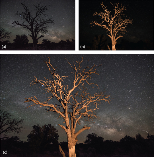
An example of this method is shown in Figure 22.5, where the two images in Figure 22.5(a and b) were blended to produce the composite image in Figure 22.5(c). The image created with the high ISO setting in Figure 22.5(a) shows remarkable detail of the Milky Way and the night sky. The image created with the low ISO setting in Figure 22.5(b), however, shows a virtually featureless night sky. Careful light painting reveals the foreground tree in the low ISO image, however, with the crisp detail and sharp definition one would expect in an image made with a low ISO setting. Blending the two together in Photoshop results in a composite image with excellent light sky detail coupled with a high-quality foreground, Figure 22.5(c).

22.5 Blending two images together, each taken at a different ISO setting, is a terrific method for extracting the best features of both. Here, the image created with the high ISO setting (a, top left) shows remarkable detail of the Milky Way and the night sky, but an extremely grainy foreground. A corresponding image created with a much lower ISO setting, (b) top right, however, shows a virtually featureless night sky but very good detail of the foreground subject, enhanced by careful light painting. Blending the two images together in Photoshop results in a composite image, (c) bottom, that shows a good level of detail in the sky, coupled with a prominent, high-definition foreground.

Blending Tracked Skies with Untracked Foregrounds

The use of a tracking equatorial amount, Figure 18.10, allows the creation of night sky images with extraordinarily long shutter speeds and virtually no star trails. Images with exposure times of several minutes in length can be routinely created. Unfortunately, as we have seen, Figure 18.11, foreground objects become undesirably blurred, as the earth now moves underneath the apparently motionless sky.

This problem is easily remedied by blending together a long exposure image of the tracked sky with a second, identically exposed image of the untracked foreground. The night sky will be sharply defined in the first exposure but the foreground will be blurry. In contrast, the night sky will be filled with streaked star trails in the second exposure, but the foreground will be sharply defined. Simply blending the sharply defined regions of both images produces a composite image with extraordinary detail. The exposure of the untracked foreground is best done last when facing east and first when facing west to avoid the potential for underexposing the sky regions in the final, blended image. The order doesn’t matter when facing either north or south, as sections of the sky will be inevitably affected in either case.

This technique was used to create an incredibly detailed image of the Milky Way rising over Mt. Boney in the Santa Monica Mountains just outside Los Angeles, California, as shown in Figure 22.6. Both images used to create the composite are also shown, Figure 22.6(a, b); each was made with a shutter speed of 4 minutes and an ISO of only 200. This low ISO setting coupled with a four-minute exposure time resulted in the unprecedented clarity of the Milky Way in this otherwise heavily light-polluted area.

Sunset/Sunrise Blending with Night Sky

Yet another technique for producing powerful nightscape images involves blending two or more images created before, during, and after sunset, as illustrated by the example shown in Figure 22.7. This example shows one of the sheets of ice that forms into piles and stacks along the north shore of Lake Superior each winter. By positioning myself between the blade of ice and the imminent sunrise, I was able to create multiple images that included the Milky Way rising in the pre-dawn astronomical twilight of late February, Figure 22.7(a–c). The composite image, Figure 22.7(d) was created by blending together different regions of individual images created at various stages of twilight using simple layer masks in Photoshop. Admittedly, the result is more a work of art than a simple photograph, and as always, it is up to you where you wish to draw the line between unalloyed documentation and artistic license.

Panoramas

Gorgeous panorama images can be obtained by combining, or “stitching,” multiple images together into a single composite image with incredible resolution. This is simply accomplished by creating a series of images with 30 to 60 percent overlap between them, Figure 22.8(a). The individual images can then be easily merged within Photoshop, Lightroom, PT Gui, or the Image Composite Editor (ICE) software freely available from Microsoft. Both single row and multi-row panoramas can be created through these techniques.

22.6 The blurry foreground (top right), present in a tracked, long-exposure nightscape, can be mitigated by combing the image with an untracked version with the same exposure settings (top left). The composite image can exhibit extraordinary detail, as shown here for the Milky Way rising over Mt. Boney in the Santa Monica Mountains just outside Los Angeles, California.

22.7 Beautiful images can be created by combining different versions of the same image but simply made at different times. This example shows a blade of ice that formed along the north shore of Lake Superior during winter. By positioning the camera between the ice blade and the imminent sunrise, I was able to create multiple images that included the Milky Way rising in the pre-dawn astronomical twilight of late February (top). The composite image (bottom) was created by blending together different regions of the top images using simple layer masks in Photoshop.

22.8 Stunning panorama images can be obtained by combining several images together. This is simply accomplished by creating a series of images with 30 to 60 percent overlap between them, as shown here in (a). These individual images can then be merged within Photoshop, Lightroom, or the Image Composite Editor (ICE) software freely available from Microsoft, as shown in (b), to produce an image with high pixel dimensions. Such images are easily enlarged to create very large prints.

There are a few precautions that should be made when creating images in preparation for the generation of a panoramic composite. First, care must be taken to use a manually focused camera with a manually set white balance and a manual exposure setting. If the focus, white balance, or exposure changes during the creation of the images, then the resultant composites will appear defective. Second, it is important to maintain a level horizon while creating the input images. This step can be assisted immensely with the help of a panoramic head, Figure 18.10. An added benefit of a panoramic head is that it keeps the axis of rotation of the camera through its nodal point as the input images are created, thus minimizing the introduction of parallax between successive images. Foreground objects can appear to shift sideways relative to the background in successive images as the result of parallax if the camera is not rotated about its nodal point. Parallax is a common source of alignment error during the merging of images created by hand, or with a simple rotating ballhead. On the other hand, if your image does not contain any nearby foreground subjects, then parallax is less of a concern.

Another issue to bear in mind while you are collecting input images to merge into a panoramic composite image is the need to act quickly. Any perceptible movement within the scene can lead to significant difficulties during the merging of the individual images. For example, clouds, the aurorae, and changes in light in general can all wreak havoc if there are substantial differences between successive images.

Finally, any lens corrections should be performed in Lightroom before merging the individual images. Lens vignetting is an especially important effect that should be eliminated before attempting to merge individual images.

Star Trails

Star trail images are ubiquitous nightscape images that are easy and fun to produce, Figure 22.9. In

22.9 Star trail images are easy and fun to make. This north-facing image was taken just outside Seventeen Seventy, Australia, and shows stars arcing from right (east) to left (west) over the northern horizon.

22.10 (a)–(f) Input images for star trails, each made 31 seconds apart. The inset, (g), shows the planet Venus, along with the short star trails captured within each image. Images such as these were used to create many of the star trail images shown in this book, for example, Figures 15.22 and 23.11; typically, hundreds of such images would be combined.

22.11 This schematic illustrates the typical timing sequence used to create a series of star trail images. The main parameters to set are the shutter speed and the intervening time required to store each image. Different manufacturers use different notations to define the interval timing parameters. In (a), the interval includes both the exposure time as well as the time needed to store the image onto the memory card. In (b), the interval simply refers to the duration of the gap between successive images.

fact, you will soon begin to “see” star trail possibilities as you journey along! The basic concept is simple: obtain multiple exposures with relatively short shutter speeds, say 5–30 seconds, Figure 22.10, and then combine them in a way that only the movements of the stars are retained. Star trail image processing can be done using any of several readily available techniques; a few of the more popular approaches are described herein.

Suitable input images can be combined, or “stacked,” to create star trails in a few different ways. Their pixel values can be simply added together, resulting in the creating of star trails as the stars move against the dark background between successive images. However, this approach will result in a badly overexposed foreground, since their values will add, too. An alternative approach is to only add together pixel values if they change by becoming brighter between successive images, for example as would be the case when a star moves into a previous dark region of the night sky. This latter approach, implemented through the “Blend – Lighten” procedure in Photoshop, for example, is at the heart of most star trail stacking algorithms.

Let’s begin by considering the practicalities of obtaining optimum star trail input images. When using the in-camera timer, or an external intervalometer, there will inevitably be at least a one second interval between successive images. This gap is the result of the amount of time required to store each image before creating the next one, Figure 22.11. Thus, if each star trail image is 4 seconds in length, then the resultant composite will suffer from gaps along 20 percent of each star trail. In contrast, if each image is 19 seconds in length, then the gaps will be reduced to only 5 percent of the total length. Examples of star trails with and without gaps are shown in Fig. 22.12.

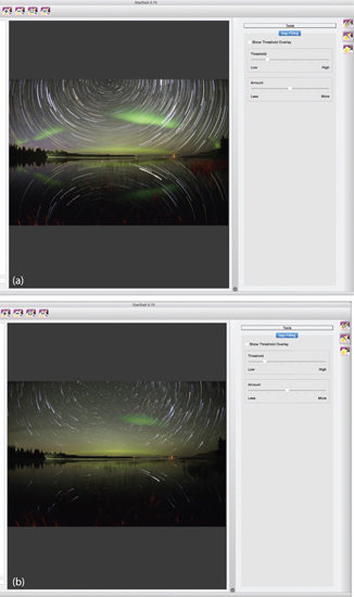
22.12 These two images show the effects of blending star trails with (a) 20 percent vs. (b) 5 percent gaps.

One way to circumvent this deficiency is to set the exposure mode to “Continuous” and to attach a locked manual shutter release cable. While the cable is attached, the camera will simply record successive images in immediate succession. Each image is held in a temporary memory buffer and stored during the exposure of the subsequent image. Finally, in either method, you may wish to make a final dark-frame image with the lens cap on for subsequent noise reduction.

The next step is to set our ISO, aperture and shutter speed. This process is aided by the case we studied in Chapter 12, e.g. Figure 12.7, where we explored the best of all the possible combinations in aperture, shutter speed, and ISO. The same questions arise in the creation of images for use in star trail stacking. Namely, of the several equivalent exposure settings, particularly those trading ISO levels off against shutter speeds, which combination is the best? Specifically, ignoring the issue of potential gaps, is it better to combine fewer exposures each made with a longer shutter speed and a lower ISO or more exposures at higher ISO made with shorter shutter speeds?

The definitive answer is that the star trail image quality is markedly superior by combining a larger number of shorter duration, high ISO exposures. This outcome is demonstrated in Figure 22.13, where three images are analyzed and compared, each made from an increasing number of nominally equivalent input images, all with identical aperture settings. The first image, Figure 22.13(a), was a single exposure at 240 seconds with an ISO setting of 100. The second

22.13 This exercise demonstrates the benefits of stacking multiple, shorter exposures at high ISO for the creation of star trails. All three images, (a)–(c), were made with the identical EV. The first image, (a), was a single exposure at 240 seconds with an ISO setting of 100. The second image, (b), stacked eight exposures with the same overall EV; each was made at 30 seconds (three EV stops lower than (a)) with an ISO of 800 (three EV stops higher than (a) to compensate). The third image, (c), stacked sixty exposures with the same overall EV as the first and second images; each made at 4 seconds (six EV stops lower than (a)) with an ISO of 6400 (six EV stops higher than (a) to compensate). There are clearly the most star trails visible in the image stacked with the sixty images at 4 seconds apiece even while its background noise level is quite low. (d) Quantitative image analysis accomplished by measuring the image intensity along the line connecting Point A and Point B, (c), in each image. The dimmer star intensity peaks increase by almost a factor of ten relative to the sky between the 240-second single image and the sixty stacked 4-second images!

image, Figure 22.13(b), stacked eight exposures with the same overall EV; each was made at 30 seconds (three EV stops lower than the first image) with an ISO of 800 (three EV stops higher than the first image to compensate). The third image, Figure 22.13(c), stacked sixty exposures with the same overall EV as the first and second images; each made at 4 seconds (six EV stops lower than the first image) with an ISO of 6400 (six EV stops higher than the first image to compensate). There are clearly the most star trails visible in the image stacked with the sixty images at 4 seconds apiece even while its background noise level is quite low.

We can further quantify this result through analysis of the resultant images, Figures 22.13 (a)–(c), using the freely available program ImageJ. ImageJ is a public domain image-processing software freely available from the National Institutes of Health (NIH), the same government agencies responsible for the nation’s medical research. Originally designed to assist with the analysis of scientific images, it can be used to edit images, create animations, and perform quantitative image analyses.

The quantitative image analysis is accomplished by measuring the image intensity along the line connecting Point A and Point B, Figure 22.13(d), in each image. This is done by: (i) opening each image within ImageJ; (ii) using the line tool to define the analysis path; and (c) executing: Analyze → Plot Profile. ImageJ then measures the image intensity along the selected analysis path and generates the graphs shown in Figure 22.13(d) for each image.

The intensity peaks in the graphs corresponding to the stars can be compared to the relative background intensity level of the sky after first adjusting the background sky level to comparable values. What can be seen is that the dimmer star intensity peaks increase by almost a factor of ten relative to the sky between the 240-second single image and the sixty stacked 4-second images! This is an enormous difference—akin to more than a three-stop improvement in EV! This example clearly demonstrates the advantages of combining a greater number of exposures with high ISO settings and shorter times than fewer exposures made at longer exposure times. Of course, larger memory cards are needed to hold all the additional images!

Let’s now discuss the various methods available to actually perform the star trail stacking. First, it is entirely possible, albeit laborious, for you to individually blend together all of your star trail images within Photoshop. All you need to do is to convert each image to a separate layer within a single image and then perform the “Lighten Blend” operation on each layer sequentially. Fortunately, Photoshop makes it easy for you to automate this process through the creation of a Photoshop action, or recorded sequence of automated tasks.

A simpler approach is to use the freely available StarStaX software. StarStaX allows you to easily convert a sequence of individual star trail images into a composite image with several options for the manner in which the star trails are created. They can be combined into solid streaks of light, Figure 22.14(a), or one or both sides of the trails can be preferentially dimmed in what is termed the “comet” mode, Figure 22.14(b). An especially useful feature of StarStax is that the processed, individual images used to create the final composite can be saved as intermediate files and then later converted into a separate time-lapse video sequence with stunning effects, as described below.

22.14 The results of combining multiple input images using StarStaX: (a) basic stacking; no special effect and (b) stacked using the “comet” mode.

Source: http://www.markusenzweiler.de/software/software.html

Another alternative is the image-stacking Photoshop script provided by Waguila Photography. Like the action described earlier, a script is a saved sequence of steps that can be performed automatically. Here, a number of options allow you to tailor the appearance of your star trail images. This method was used to create the image shown in Figure 15.22.

One undesirable side effect of stacking numerous images is the inevitable accumulation of all the hot pixels from each image. Unless these are removed from each image before stacking, the only alternative is to laboriously remove them from the final, stacked image. Airplane and satellite lights are another set of artifacts that should be removed prior to image stacking. Great care must be exercised in doing so, however, to avoid removing nearby stars and thus unintentionally introducing gaps in the resultant star trails.

Meteor Shower Composites

Meteor showers are named after the constellation from which they appear to originate; i.e. where their radiant point is located, as described in Chapter 7. Beautiful images can be made with single meteors, Figure 22.15. Care must be taken to ensure that what appears to be a meteor is, in fact, a meteor. Satellites, airplanes, and Iridium flares can occasionally be mistaken for meteors.

22.15 A lone meteor example streaks across the sky over Devils Tower and next to the Milky Way during the 2015 Perseid meteor shower.

The distinguishing characteristics of a meteor are its containment within a single image, its linear shape, and varied colors from end-to-end. If the object suspected of being a meteor spans two images, or exhibits gaps, then it is not a meteor but another object.

Selecting individual meteors from separate images obtained throughout a single meteor shower, and combining them together, can yield a beautiful composite image. Producing it is relatively straightforward; a significant issue, however is the movement of the stars that occurs during the typically several hours of exposure necessary to capture several meteors. This movement must be corrected for in order to produce an image (a) without star trails and (b) with all the meteors correctly appearing to originate from the radiant. Here’s how this is done.

First, be sure your composition contains a celestial pole. If it doesn’t, then this alignment technique will not work. The Perseid meteor shower is especially conducive to this approach, since its radiant point is relatively close to Polaris. Next review each image carefully to select those containing a meteor. Separate the meteor-containing images into a distinguishable group.

Pick one of the meteor-containing images to be the image into which all the meteors from the other images will be merged. We will call this the foundation image. You will likely want to select the foundation image to be the one corresponding to the time when the radiant point is the highest in the sky. This will best convey this sense that the meteors are raining down from above.

Open the foundation image and one of the other meteor-containing images in Photoshop, Figure 22.16(a). Copy the second image as a separate layer in the first image. Combine both layers using the “Light Blend” command, Figure 22.16(b). You will see the relative motion of the stars around the celestial pole as miniature star trails. Repeat these steps with the remaining meteor-containing images; when you’re done, you will have an image with distant star trails encircling the celestial pole. Create another layer and use it to mark the point of the celestial pole. Keep this layer visible and uncheck the visibility of all but the foundation image layer and one of the remaining layers.

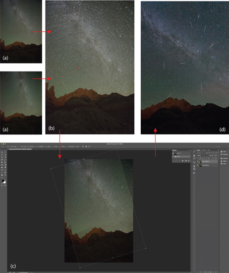
22.16 Brilliant meteor shower composite images are straightforward, if time-consuming, to make. First, be sure your composition contains a celestial pole. Pick one of the meteor-containing images for the foundation image. Open it and another meteor-containing image in Photoshop, (a). Copy the second image as a separate layer in the first image. Combine both layers using the “Light Blend” command, (b). You will see the relative motion of the stars around the celestial pole as miniature star trails. Repeat these steps with the remaining meteor-containing images; when you’re done, you will have an image with distant star trails encircling the celestial pole. Create another layer and use it to mark the point of the celestial pole. Keep this layer visible and uncheck the visibility of all but the foundation image layer and one of the remaining layers. The next step is to rotate the second layer around the celestial pole to bring it back into alignment with the foundation image, (c). This is easily done in Photoshop using the rotate command and moving the center of rotation to the point marking the celestial pole. Once this is done, simply select just the meteor from the second layer using a mask, and discard the rest of the layer. Repeat these steps with the other layers until you’re left with a single, composite image containing the correctly aligned meteor from each of the meteor-containing images, (d).

The next step is to rotate the second layer around the celestial pole to bring the sky in this image back into alignment with the sky in the foundation image, Figure 22.16(c). This is easily done in Photoshop using the rotate command and moving the center of rotation to the point marking the celestial pole. Once this is done, simply select just the meteor from the second layer using a mask and discard the rest of the layer. Repeat these steps with the other layers until you’re left with a single, composite image containing the correctly aligned meteor from each of the meteor-containing images, Figure 22.16(d).

Time-Lapse Video

A burgeoning frontier of landscape astrophotography involves the creation of beautiful time-lapse videos. These are remarkably simple to make using tools that you likely already have, or can download for free. Photoshop has an option to easily create a video from a series of images. All that is required is to open the first image in the sequence, after checking the small box titled, “Image Sequence,” in the pop-up dialogue box. After the first image is opened, the “Render Video” command is executed from the “File” menu and the video is automatically created. ImageJ can also be used to create basic videos from a sequence of input files in a similar fashion.

One other program for creating time-lapse videos deserves special mention—LRTimelapse, which was developed specifically with the landscape astrophotographer in mind. It is available in a scaled-down, free trial version that allows you to create a time-lapse video from up to 400 input images, enough to allow you to decide whether you wish to invest in it.

LRTimelapse offers several powerful features that are essential for the best quality time-lapses. One of these is a sophisticated “de-flicker” algorithm. This tool effectively eliminates the minor, but perceptible fluctuations in exposure between successive frames that inevitably result from tiny differences in the actual positions achieved by the individual blades of the aperture diaphragm, even at a constant aperture setting. As the diaphragm opens and closes between each frame in a time-lapse sequence, the diaphragm blades come to rest at minutely different positions, creating subtle differences in the aperture between successive images. The differences in aperture result in barely perceptible differences in exposure between successive images. During the accelerated playback of a time-lapse sequence, however, these differences in exposure manifest themselves as a noticeable flickering. The LRTimelapse de-flicker tool allows the user to smooth out these tiny differences almost completely.

LRTimelapse is also remarkably effective at helping create the so-called “Holy Grail” time-lapse sequences. Its underlying strategy is to identify a handful of images throughout the sequence that it labels as “key frames.” Each key frame is selected from a specific point during the holy grail sequence. The first key frame is usually the first image in the sequence, and the final key frame is usually taken near the end of the sequence. The intervening set of key frames are selected to encompass the range of exposures. The user then edits each key frame separately in Adobe Lightroom to achieve the desired appearance. The key frames are then brought back into LRTimelapse and after a few subsequent steps where the exposures of the entire sequence are adjusted according to the exposures of the key frames, the entire sequence is then exported into a video. The entire process is quite straightforward and enables the user to create truly spectacular time-lapse videos of nightscapes.

Concluding Remarks

This section has focused on the possibilities enabled by combining multiple images into a single, composite result. Images produced through these techniques can be simply astonishing! Now, however, I don’t wish in any way to devalue the incredible satisfaction of achieving single-exposure nightscapes that demand expert levels of proficiency in all the subjects described in this book. As you will see in the case studies, for example, such images may take years to create! They can require skilled application of techniques in wilderness environments whose special secrets can be slow to reveal themselves. There is an immense amount of pride in making one of these single-exposure images. They offer evidence of advanced photographic credibility, the joy of witnessing a transient moment of perfection, and the satisfaction of meeting demanding dual photographic and astronomical challenges. Nonetheless, multiple-image nightscapes simply represent yet another avenue of artistic and scientific exploration; both promise a lifetime of worthwhile pursuit.