You can process various objects in SSAS: databases, cubes, dimensions, measure groups, partitions, data mining models, and data mining structures. When you process an object, all the child objects are reviewed for processing. If they are in an unprocessed state, they are then processed as well.

To process the Adventure Works cube, select Process... from the Adventure Works.cube context menu, or click Process in the cube designer toolbar. This will display the Process Cube dialog, as shown in Figure 13-1.

Figure 13.1. The Processing dialog

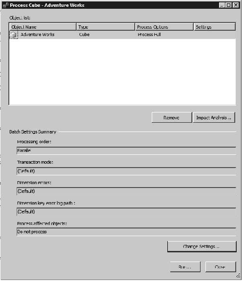
How the cube will be processed depends on the processing option selected. You have the following options available via the Process Options drop-down list:

Clicking the Change Settings button will open the Change Settings dialog, which has two tabs, Processing options and Dimension key errors. In this section I'll focus on the Processing options tab, which is shown in Figure 13-2.

Figure 13.2. The processing settings dialog

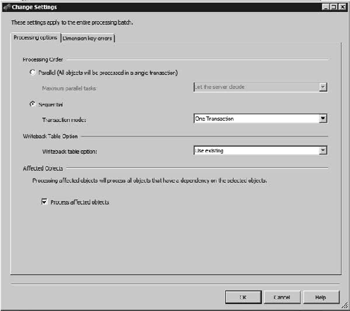
Under Processing options you can select whether to process the objects in parallel or sequentially. Parallel processing splits a task and allows jobs to run in parallel. However, during parallel processing, objects will be taken offline as they're processed. The result is that the cubes will be unavailable during most of the processing process. Parallel processing is wrapped in a single transaction, so if the processing fails, all the changes are rolled back.

Sequential processing has two options: One Transaction or Separate Transactions. When processing an SSAS job as a single transaction, the entire task is wrapped in a transaction—if there's an error at any time during processing, the whole thing is rolled back. The major benefit is that the cube stays available to users until the transaction is committed, at which point the whole update is slammed in place at once.

If you process a task as separate transactions, each job is wrapped in its own transaction, and each is committed as they're completed. The benefit here is that if you have a large, complex processing task, it can be painful to have the whole thing roll back because of one bad piece of data. Processing a series of jobs sequentially as separate transactions means everything up to the error will be kept—only the current job will roll back.

Writeback tables are also something you can configure from the Processing options tab. Writeback tables are relational tables created when you enable writeback on a partition. Certain changes to cube structure can invalidate the writeback tables if they no longer map to the cube structure. The Writeback Table Option indicates what processing should do with existing writeback tables.

Finally, Process Affected Objects will process objects that have a dependency on objects being processed. For example, if you process a dimension and select this option, the cubes that depend on that dimension will also be processed.

So let's take a look at the mechanics of processing an object in Analysis Services, which I feel helps reinforce the understanding of what's going on behind the curtain.

When Analysis Services processes a cube, the end result is a number of binary hash files on disk for the dimensions, attributes, and aggregates generated to optimize response time for dimensional queries. How do we get from a collection of .xml files that define the cube to the processed hashed binary files that are the cube?

When you issue a process command, the Analysis Server analyzes the command, and evaluates the objects affected and their dependencies. From that the processing engine will build a list of jobs to be executed and their dependencies. The jobs are then processed by a job execution engine, which performs the tasks necessary to build the file structures for the cube. Jobs without dependencies on each other can be executed in parallel. The server property CoordinatorExecutionMode controls how many jobs can run in parallel at once.

A dimension-processing job will create jobs to build the attribute stores, creating the relationship store, name, and key stores. The Attribute job will then build the hierarchy stores, and, at the same time, the decoding stores, followed by bitmap indexes on the decoding stores. As the attribute-store processing job is the first step, it's the bottleneck in processing; this is why having a well-structured attribute relationship is so important.

The decoding stores are how the storage engine retrieves data for the attributes in a hierarchy. For example, to find the part number, price, and picture of a specific bicycle, the storage engine fetches them from the decoding stores. The bitmap indexes are used to find the attribute data in the relationship store. The processing engine can spend a lot of time building the bitmap indexes while processing, especially in dimensions with a large number of members. If a collection of attributes is unique, the processing engine may spend more time building bitmap indexes than they're worth.

A cube-processing job will create child jobs for measure groups, and measure-group jobs will create child jobs for partitions. Finally, partition jobs will create child jobs to process fact data and build the aggregations and bitmap indexes. To process the fact data, the job-execution engine queries the data sources from the data-source view to retrieve the relational data. Then it determines the appropriate keys from the dimension stores for each relational record and populates them in the processing buffer. Finally, the processing buffer is written out to disk.

Once the fact data is in place, then jobs are launched to build the aggregations and bitmap indexes. They scan the fact data in the cube matrix, then create the bitmap indexes in memory, writing them out to disk segment by segment. Finally, using the bitmap indexes and the fact data, the job engine will build the aggregations and aggregation indexes in memory, writing them out to disk when they're complete.

Your first tool in evaluating the processing of a cube is the SQL Server Profiler. Profiler is an application that allows you to log all events being performed on or by a SQL Server service. In the case of Analysis Services, we want to run a trace on SSAS while performing an action of interest (in this case, processing a cube.) Figure 13-3 shows part of a trace from a cube-processing job. From the Profiler trace, you can identify the start time and completion time of various tasks, and from there figure out how long various tasks are taking, and, more importantly, where most of the time is being spent processing.

Figure 13.3. Profiler trace from Analysis Services while processing a cube

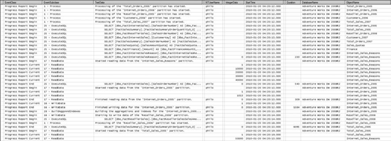
Another use for Profiler is to watch the relational store while processing. While Analysis Services is building cubes and dimensions, any data it needs from SQL Server it retrieves via query. You can watch these queries via a Profiler trace on the relational store and again identify where the bottlenecks are. The SQL used for the queries is reported there, and you can run Query Analyzer on the queries to ensure they're as efficient as possible.

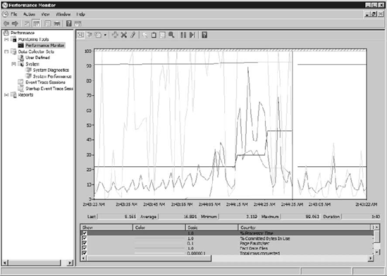
Windows Performance Monitor (found in Administrative Tools on the Start Menu) is a tool that provides resources for analyzing system performance. Figure 13-4 shows an analysis in progress. You can analyze operating systems, server software, and hardware performance in real time, collect data in logs, create reports, set alerts, and view past data. The metrics tracked by Performance Monitor are performance counters. Windows comes with hundreds of counters built in (for disk performance, CPU, memory, caching, and so on). Third-party software, as well as other software from Microsoft, can install additional performance counters.

Figure 13.4. Windows Server 2008 R2 Performance Monitor

When you install Analysis Services, it adds a number of new counter groups:

Each of the counter groups will have a number of counters subordinate to them. For example, MSAS 2008:Processing has six counters for reading, writing, and converting rows of data. By tracking certain performance counters you can evaluate the performance of your Analysis Services server. If you're getting complaints of bogged-down performance that you can't pin down, you can run the performance counters to a log file for review later. For more information about the Windows Performance Monitor, check out the TechNet article at http://technet.microsoft.com/en-us/library/cc749249.aspx.

Once you have an Analysis Services database in production, you will need to process the cube periodically to refresh it. Remember that only ROLAP partitions and dimensions will dynamically show changes in the underlying data, so if we expect the data in the data sources to change, the cube will have to be processed to reflect the changes.

For active partitions, you will have to decide on a processing schedule depending on the business requirements. For example, cubes that are used for strategic analysis may need to be processed only once a week, as the focus is on the previous year at the quarterly level. On the other hand, a project manager may want analytic data to be no more than 24 hours old, as it provides data for her project dashboard, which she relies on heavily on a daily basis. Finally, archive partitions for previous years may be able to sit untouched for long periods of time, being proactively reprocessed should the underlying data change.

In any event, all these requirements indicate a need for automated processing. The good news is that there is a lot of flexibility in the processing of SSAS objects. Essentially, there are two ways to initiate the process: either via an XMLA query, or by calling the AMO object model. However, we have a number of ways to accomplish those two tasks.

You can process Analysis Services objects with XML for Analysis (XMLA) queries. This means that essentially any tool that can connect to SSAS and issue a query can process objects, if that connection has the appropriate privileges. One great benefit is that if you want a cube or database processed a certain way, you can create the script and store it separately, then use the same script to process the object(s) manually, through code, via tools, and so on.

A basic example is shown here, but the processing options in XMLA are full-featured enough to duplicate anything you can do through the BIDS UI.

<process xmlns="http://schemas.microsoft.com/analysisservices/2003/engine">
   <Object>
      <DatabaseID>Adventure Works DW</DatabaseID>
      <CubeID>Adventure Works</CubeID>
   </Object>
   <Type>ProcessFull</Type>
   <WriteBackTableCreation>UseExisting</WriteBackTableCreation>
</Process>

You can fire off multiple tasks in parallel by using the <Batch> XMLA command. SSAS will attempt to execute as many multiple statements within a <Batch> command in parallel as possible, and, of course, execution will hold at the end of the <Batch> command until all subordinate commands are completed.

For more information about processing SSAS objects with XMLA queries, check the TechNet article at http://technet.microsoft.com/en-us/library/ms187199.aspx.

Analysis Management Objects (AMO) are the members of the Microsoft.AnalysisServices class library that provide for the automation of Analysis Services. Working with Analysis Services objects via AMO is very straightforward. (I'll cut to the chase—the code to process a cube is Cube.Process(ProcessType.ProcessFull)—startling, isn't it?) The upside to using AMO is that it's very intuitive, and the .NET code can make it easy to perform some pretty arcane tasks.

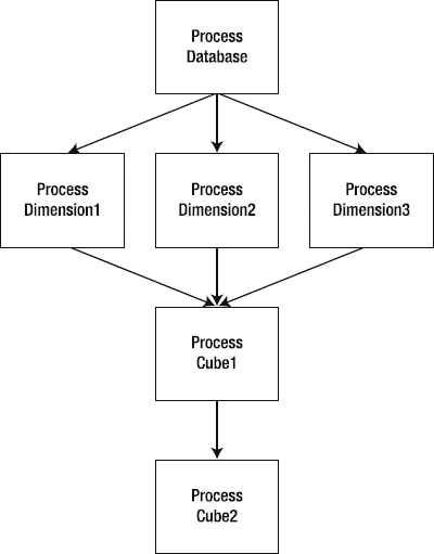
For example, consider a complex Analysis Services database that has various dependencies, and you want to enable your users to request a cube to be reprocessed. For a given cube, there are various dimensions that need to be reprocessed, depending on when it was last processed and the age of the data. Now if the structure of what needs to be processed in which order is static, similar to what's shown in Figure 13-5, then creating the process job in XMLA makes sense—structure the query once, and store it.

Figure 13.5. Simple execution of a batch process

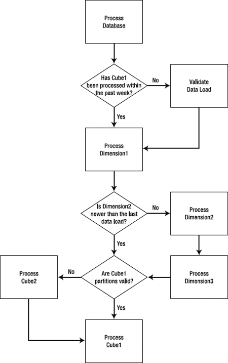
When you have a complex cube structure, you may want to create specific dependencies (if you process x dimension, then process y cube). You may also want to verify partition structures, data freshness, or even compare the last processing data against the age of the data to determine if you need to reprocess an object. So you may end up with a process similar to that in the flow chart shown in Figure 13-6. In this case, it may make more sense to craft the reprocessing logic in code. It's going to be easier to trace the flow through code, and it will be easier to instrument and debug.

Figure 13.6. A notional complex logic flow for processing a database

The code is very straightforward:

Server server;
Database db=new Database();

//connect to analysis server
server = new Server();
server.Connect(@"data source=<server name>");
db = server.Databases["<database name>"];

foreach(Cube cube in db.Cubes)
{
    //Processes cube and child objects
    cube.Process(ProcessType.ProcessFull);
}

Remember that cubes own measure groups; dimensions are owned by the database.

A common problem when dealing with automation is the need for a framework to run the code in. Very often you may find the easiest way to tackle an administrative task is with code, but you end up taking the time to create a small application to run the code. And next time you need to run the code, you don't have the application handy, so you have to do it again.

In the Unix world, this is rarely a problem—since everything is command-line interface, then any administrative task can usually be performed by writing a script. Windows administrators didn't really have this option for a long time—there wasn't anything between 1980s-era batch files and modern fourth generation code. That is, until Microsoft created PowerShell.

PowerShell is a Windows component introduced a few years ago to enable scripting for enterprise applications. It works very similar to scripting shells in Unix, with the exception that instead of piping text from one process to another, PowerShell enables passing actual objects from one to the next. It's available as a download for Windows XP, Vista, and Server 2003, and is an installable component with Windows 7 and Server 2008 and 2008R2.

Since PowerShell can leverage .NET assemblies, the code in PowerShell will be similar to the .NET code in the previous section. The benefit here is that you can write and execute that code against an Analysis Services server without having to build a harness or application for it. You can learn more about PowerShell at http://technet.microsoft.com/en-us/scriptcenter/dd742419.aspx.

Now that we have a solid collection of ways to automate processing of Analysis Services objects, we need a way to kick it off. Perhaps we need to trigger the processing on a regular schedule, or we want to call it when we load data into the data mart. Alternatively, it's possible that we don't have control over the data-loading process, and need to trigger processing when data in a warehouse changes.

We're going to take a look at SQL Server Agent, a process that runs in SQL Server and can be used to schedule cube processing. We'll also take a look at SQL Server Integration Services—the primary use of SSIS is to extract, transform, and load (ETL) data; it's often used to load data warehouses from production systems. Since SSIS is doing the loading, it can also trigger or schedule the processing of the affected objects in Analysis Services.

SQL Server Agent

SQL Server Agent is a component of SQL Server, and runs as a Windows Service. You can configure SQL Server Agent either through T-SQL or via SQL Server Management Studio, as shown in Figure 13-7.

Figure 13.7. Managing SQL Server Agent through SSMS

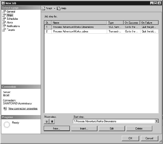
Each job can contain a number of steps, as shown in Figure 13-8, and for each step you can indicate what action to take depending on whether the job step exits reporting success or failure (exit the job, reporting success or failure, or continue on to the next step). Each step can also write to an output file, log results to a table, or place its results in the job history. You can also set the user context for each specific job step.

Figure 13.8. Creating a job for the SQL Server Agent

Job steps can be a number of things, each option having its own options for execution. While there are twelve different types of job steps, the ones we're interested in are PowerShell, SQL Server Analysis Services Command, and SQL Server Analysis Services Query. As you can see from the methods we've covered previously, these options allow us to schedule Analysis Services processing jobs by calling a PowerShell script, running an XMLA query, or using the Analysis Services command directly.

Once we have the processing job set up the way we want, then we can select or build a schedule, and set up the alerts and notifications we want to execute when the job finishes.

While the SQL Server Agent is the best way to schedule a recurring action you want to perform on Analysis Services, if you need actions executed as part of a process, your best bet is SQL Server Integration Services (SSIS). There's a good chance that in an Analysis Services BI solution, you'll be using SSIS to move data into your data mart or data warehouse. The nice thing is that while using SSIS to move data (which means you'll need to reprocess the cubes and/or dimensions at some point), you can also trigger the reprocessing directly.

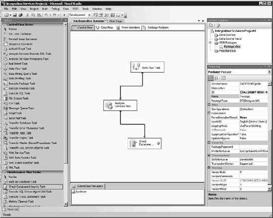
SSIS uses a drag-and-drop designer for data-oriented workflows, as shown in Figure 13-9. For an ETL type job, the central point of the workflow will be the Data Flow Task, which contains logic for moving and transforming data. However, in the Control Flow, there is a task for processing Analysis Services objects.

Figure 13.9. SQL Server Integration Services designer in BIDS

You can make paths conditional, so as we've discussed, you may want to process cubes only when the underlying data has changed. You can also have different exit paths based on success or failure of the previous component. This is beneficial if a data load job fails—you don't want to waste downtime either processing a cube on unchanged data, or, worse, processing a cube on bad data.

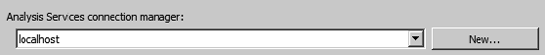
Configuration of the Analysis Services task is very straightforward. First you need to create a connection to the Analysis Server, either by right-clicking in the connection manager pane and selecting New Analysis Services Connection or by opening the properties pane of the Analysis Services Processing Task and clicking New next to the connection manager selection drop-down list, as shown in Figure 13-10.

Figure 13.10. Selecting a connection to Analysis Services

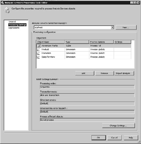
The processing settings themselves reflect the settings dialog we're familiar with, as shown in Figure 13-11. Once you select the connection manager, then you will be able to add objects from the database selected in the connection manager. You can select cubes, measure groups, partitions, dimensions, or mining models. Once the selections are listed in the dialog, you can change the processing settings for each object individually.

Figure 13.11. Processing settings in SSIS

The green arrow from the bottom of the task leads to the next task you want completed. You can have multiple arrows leading to multiple tasks, and the arrows can be configured to be conditional based on the success or failure of the task, or more intricately based on an expression, which may depend on variables defined in the Integration Services package.

If you're interested in learning more about Integration Services, I highly recommend the Integration Services tutorials online at http://msdn.microsoft.com/en-us/library/ms167031.aspx. You can also read more about SSIS in SQL Server 2008 Integration Services Unleashed (Sams, February 2009) by Kirk Haselden, one of the SSIS architects at Microsoft.

A few times I've referred to security and permissions with respect to working with Analysis Services. Due to the sensitive nature of both the information contained in SSAS cubes and the data that underlies them, implementing security properly is of paramount importance. Let's take a look at some aspects of security in SSIS.

Analysis Services recognizes only Windows Integrated Authentication, also known as Active Directory security. As of SQL Server 2008 R2, there is no other authentication method available. With respect to connecting from the Internet, this can be problematic, as generally your firewalls won't have the necessary ports open for NT authentication. In this case you can configure SSAS for HTTP access, which uses an ISAPI filter to connect to SSAS from IIS on the web server.

HTTP access can be performed with any authentication mode on IIS—NTLM, Basic (username/password), or even anonymously (using the IIS application pool account to authenticate into SSAS). The general architecture and authentication flow will look like Figure 13-12. A great article regarding setting up HTTP access for SQL Server 2008 Analysis Services on Windows Server 2008 can be found at http://bloggingabout.net/blogs/mglaser/archive/2008/08/15/configuring-http-access-to-sql-server-2008-analysis-services-on-microsoft-windows-server-2008.aspx.

Figure 13.12. User authenticating against Web application

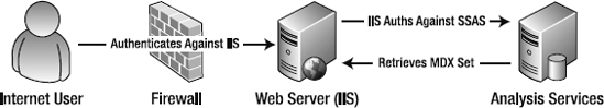
However, don't be in a rush to expose SSAS to the Internet in this manner—remember that you are exposing a bare XMLA query interface (so the Internet user can use Excel or another Analysis tool). If, on the other hand, you will be delivering only analytic data to Internet users via an application (Reporting Services, Excel Services, PerformancePoint, etc.), then you need to provide only for that application's authentication of Internet users, then handle authentication of the application against Analysis Services. (Again, if you choose to pass through user credentials, be mindful of the double-hop problem.)

Once we've authenticated against an Analysis Services server, then we have to do something. What we're allowed to do depends on what Authorization our user is granted. Within SSAS, authorization is handled via role-based security—roles are objects in Analysis Services that are containers for the permissions that users authenticated into the server will receive.

Roles are defined near the bottom of the tree in the Solution Explorer pane—if you right-click on the Roles folder, you can create a new role. New roles default to not having any permissions. When you create a new role, you'll see the General tab for the role, as shown in Figure 13-13.

Figure 13.13. The General tab for a newly created role

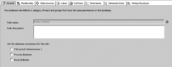
The Role name: in this tab is not directly editable. To change the name of the role, you use the Name input area in the Properties pane. The Role description: is a free-text description that allows you to annotate the intent behind the role. Then you have three checkboxes—Full Control (Administrator), Process database, and Read definition. These are fairly self-explanatory. You will want to create an Administrator role early on and get used to using that for administrators. By default SSAS creates a Server role behind the scenes—this role has administrator privileges, and has the members of the local administrators group as members. If you want to remove the local administrators from this role, you'll have to go into Management Studio and connect to the Analysis Server. Then right-click on the server itself and select Properties to open the server properties dialog.

At the bottom of the dialog is a checkbox for "Show Advanced (All) Properties." Check this to show a security property titled "Security BuiltinAdminsAreServerAdmins." If you change the value of this to "false" then built-in admins will no longer have access to the server. You can explicitly add users to the Server role on the Security tab of the Server Properties dialog.

The Membership tab is pretty self-explanatory—you can add Windows users or security groups here. The Data Sources tab controls access to the data sources in the UDM for the database. The Access property allows users to read data from the data source directly—this is used mostly in actions or drilling through to underlying data. The Read Definition checkbox will allow a role to read the definition (including the connection string and any embedded passwords!) for a data source.

The Cubes tab lists the cubes in the database and the associated access rights. Access is None for no access, and Read to allow members of the role to read the cube (which translates to "the dimensions and measure groups that belong to the cube"). Read/Write enables reading, but also writeback for the cube. The Local Cube/Drillthrough Access option for a cube allows the role to drill-through to underlying data for a cube, while a local cube allows members of the role to pull a subset of data from the cube to create a cube on their workstation. Finally, the Process checkbox, of course, allows members of the role to process the cube. You can see here that it would be possible to set up an account that has permission only to process cubes without reading any of the data—a solid security option for unattended accounts.

The Cell Data tab allows you to create fine-grained access permission on the data in a cube. There are three sections—reading cube content, reading/writing cube content, and contingent cell content. I'll explain read-contingent in a moment.

For each of these sections, when you enable the permissions, the formula box will be enabled, as well as the builder button [...] for editing the MDX. In each permission set you can directly define what cells the role has access to with an MDX expression. For example, you might want a certain analyst to have access only to mountain bikes that don't have a promotion going on. When we get to dimension security you'll see that the permissions are additive, so selecting the [Mountain Bike] dimension member and the [No Promotion] member would be overly inclusive. So instead we can use the Cell Data read permission and enter MDX for {[Mountain Bike], [No Promotion]}, which will be the set of those members we're looking for.

A potential problem here, and with dimension security, is that in some cases data that should be secured can be inferred. For example, we may allow a role to see Profit and Revenue data, but not Expenses. However, by seeing profits and revenues, you can calculate expenses through some simple math. Read-contingent permissions address this problem by digging into the constituent data under cell data—a role with read-contingent permissions is allowed access only to measures when that role is also allowed access to all the subordinate data.

The Dimensions tab is pretty basic—simply select the dimensions that the role should have access to. After selecting dimensions here, your next stop is the Dimension Data tab. Here you can select individual members of dimensions to make available to the role. You can either explicitly select and deselect members, or click on the Advanced tab and write MDX to indicate which members should be allowed or denied. You will also want to indicate a dynamic default member to align with the dynamic selections you're making.

Behind the scenes, Analysis Services uses a feature called autoexists to ensure consistent visibility of members in the hierarchies within a dimension. For example, suppose that within the Product Line hierarchy of the Products dimension you removed access to the Road member, so the role you're working on can't see any products in the Road product line. If you then looked at the Model hierarchy, you would see that no road bikes are listed. Huh? We didn't touch the Model hierarchy—so why is it filtered?

Autoexists runs against a dimension that has attribute security applied. When the cube is processed, Analysis Services will run the cross-product of all the hierarchies in the dimension, and any members wholly encompassed by a hierarchy member that is hidden from the role will also be hidden. So since all road bikes sold are in the Road product line, and the Road models in the Model hierarchy are all contained within specific members, those members are also hidden.

However, note that this cross-protection of members occurs only within the dimension where the attribute security is defined. Let's say that only road bikes were sold in 2003. If we look at sales data, we won't see the year 2003, since, with respect to the security of the role we're in, nothing we're allowed to see was sold in 2003. But that's because NONEMPTY is included in MDX queries by default. If we disable the NONEMPTY behavior, then 2003 will show up just fine (albeit with an empty cell of data).

The Dimension Data tab is also where you can set dimension members based on dynamic conditions. For example, you may want a manager to see pay data only for those employees working for him. Or you may want project managers to see only their own projects. Instead of hard-coding these selections, you can enter an MDX expression in the Allowed member set box, which will select those members dynamically based on the expression.

A more complex situation is when you want to secure a selection of members based on the logged-in user. For example, you may want users to see the sales only from the Promotions they are assigned. There are two approaches here:

Working with this type of detailed security is often a critical business requirement, but the architecture must be very carefully designed with consideration for maintainability (don't create additional data stores if you don't have to) and scalability (mapping user roles to millions of dimension members can get expensive quickly when processing or querying a cube). And on that note, let's take a look at performance considerations in SSAS.

The absolute first and foremost principle in designing for performance is "don't put it in the cube unless you need it." While it may seem prudent to be over-inclusive when deciding on dimensions, attributes, and measures, consider the impact that these will have on the cube performance. Be aware that extra measures can increase the size of the cube arithmetically; additional attributes will increase the number of cells in a cube geometrically; additional dimensions can increase the size of the cube logarithmically.

Attribute Design

In any guide to Analysis Services scalability, the top recommendation you're going to find is to ensure your attribute relationships in dimensions are properly defined. In SQL Server 2005 Analysis Services, attribute relationship design was a bit of an arcane art. However, in SSAS 2008, there is a new attribute relationship designer, as shown in Figure 13-14.

Figure 13.14. BIDS Attribute Designer

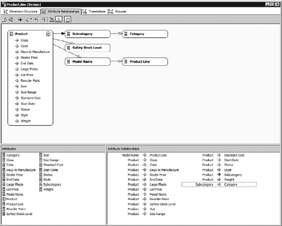
For maximum performance, create all your necessary attribute relationships—wherever they exist in the data or the model. It's also important to think in terms of good design practices for attributes. Attribute relationships direct Analysis Services on optimizing storage of data, are reflected in MDX queries, structure the presence of member properties, and govern referential integrity within a given dimension. Attribute relationships also make processing and queries more efficient, since a strong hierarchy results in a smaller hash table—top level attributes can be inferred instead of having to be discretely stored.

Attribute relationships are also the foundation on which you build hierarchies, which we've seen over and over again to be critical in the proper development of an OLAP solution. Hierarchies make it easier for end users to make sense of their data, and attribute relationships will ensure your hierarchy and the data structure make sense.

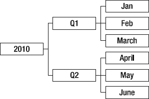
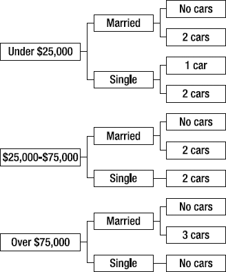
The first step in good attribute design is to observe natural hierarchies, for example, the standard calendar Year – Quarter – Month – Day, or geographic Country – State – County, as shown in Figure 13-15. Be sure that each step in the relationship is truly 1:n. You can create hierarchies that aren't a pyramid structure—these are referred to as "unnatural hierarchies," as shown in Figure 13-16.

Figure 13.15. A natural hierarchy

Figure 13.16. An unnatural hierarchy

This distinction between natural and unnatural hierarchies is important to be aware of because natural hierarchies will be materialized and written to disk when the dimension is processed. However, unnatural hierarchies are created on the fly when queried. Essentially, even when you build an unnatural hierarchy into the dimension, during execution Analysis Services treats it as if it were built on the fly. (This isn't to say not to build them, but rather that they don't benefit performance.)

Note

See Chapter 6 for more information on Attribute design.

Partitions

We've talked about designing dimensions to provide performance and scalability. How about measure groups? The most important factor in making a cube scalable is being able to partition the data. (Note that partitions are features of cubes, which consist of measure groups; they do not apply to dimensions.)

The reasons for using multiple partitions include:

• Partitions can be added, deleted, and processed independently. The primary example of this is any measure group that's having data added on a rolling basis—you can process the "current" partition at any time and the "historical" partitions remain accessible. In addition, since there's less data to scan, processing is faster.

• Partitions can have different storage settings. Considering the preceding example, the historical data can be stored in a MOLAP mode for best performance, while the current data partition can be set to HOLAP or even ROLAP so that it processes faster and reflects more up-to-date data. In addition, you can set the storage settings on various partitions, so partitions can be stored on separate servers—keep the current data local, and partition out the historical data to a remote server.

• Partitions can be processed in parallel, maximizing usage of multiple processors.

• Queries will be isolated to the relevant partitions. So if a user is querying data that happens to be from a single partition, the cube will be more responsive as there is less data to scan.

A partition is automatically created for every measure group, with that partition group containing all the records of the measure group. You can go into the Partitions tab of the cube designer in BIDS (shown in Figure 13-17) and create additional partitions if you desire.

Figure 13.17. The Partitions tab in BIDS

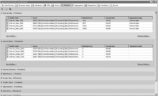
Each measure group has a section listing the partitions in that measure group. You can see that each partition has a name, and the storage mode indicated. We'll talk about the Aggregation Design in the next section. The partition will also show the estimated rows of data in that partition (you should try to keep fewer than twenty million rows of data in each partition, but this is a guideline, not a hard rule). Remember that more partitions means more files, so it's a balancing act.

The actual partitioning scheme is described in the "Source" column. This is a query that acts against the underlying table to select the specific records for the partition, as shown in Figure 13-18. The Binding type has two options: Query Binding, as shown, and Table Binding. Table Binding operates on the premise that you have a data source that is already partitioned (or perhaps you're using a view), so all that needs to be done is to select the table. Another possibility is that you can create a partition for each measure in a measure group, and those measures may come from different tables. Then you can simply create a partition for each table that contains measure data.

Query Binding, on the other hand, allows you to enter a SQL Query to select the necessary records. You can see in the partition for Internet_Sales_2007 that the query is simply all the fields in the table, and a WHERE clause limiting the results by a date range.

Figure 13.18. Selecting records for a partition

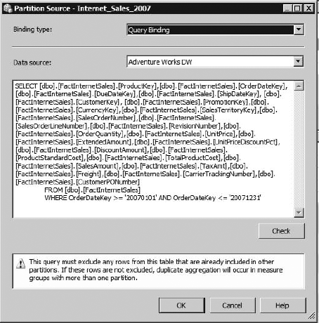
Two very important notes regarding the query—first, as the warning in the dialog indicates, be positive of your logic in the query, so that the record sets in each partition are truly unique and don't overlap. Also, if you're using a numeric range to divide the table, double- and triple-check your comparison operators—that if one partition uses < DATE, the next partition uses >=DATE, and so on. Leaving off that equals sign means you've dropped a day from your cube.

You can use multiple criteria to create partitions. For example, in addition to the calendar year divisions shown in the Internet Sales measure group, you might want to partition also by country. Then you could conceivably locate the partition for a country in the sales office for that country—queries against local data would be quick; global queries would travel the WAN and take more time. (In all honesty, in a global organization like that, you would probably be more interested in using replication, but I hope it illustrated the point.)

The two links under the partition list are to create a new partition, and to change the storage settings for the currently selected partition. The storage settings are the familiar ROLAP-MOLAP slider, and the custom settings for notifications. Set the storage location of the partition in the partition settings panel (generally on the lower right of BIDS).

The New Partition link opens the New Partition Wizard, which will walk you through creating a new partition. In the Internet Sales measure group, the group is partitioned by calendar year, so at the beginning (or soon thereafter) of each year, the DBA will have to come in, change the query on the last partition (which should be open-ended: >=0101YEAR) to add the end date for the year, and then add a new partition for the new year.

Tip

Always leave your last partition open-ended, so that in the event someone doesn't create the new year's partition in the first week of January, the users aren't stumped because none of their reports are changing.

Finally, be sure to define the slice of the partitions you create. A property of the partition, the slice is the tuple (in MDX terms) that tells Analysis Services what data will be found in each partition. For example, the partition containing the data for the calendar year of 2007 would have a slice of [Date].[Calendar].[Calendar Year].&[2007]. If the slice you enter doesn't match the data specified in the Source, SSAS will throw an error on processing.

We've learned that OLAP and Analysis Services are all about aggregating data. When we process a cube, Analysis Services will pre-calculate a certain number of aggregated totals in advance. This caching of totals helps query performance. However, SSAS won't calculate every total in advance—the number of possible combinations generally makes that prohibitive. Also, when you consider that user queries aren't going to need every single possible combination, pre-calculating everything "just in case" is counter-productive. So SSAS does a "best guess" for the amount of advance work necessary for a given cube.

Understanding Aggregations

Consider a cube with dimensions for Geography, Products, and Time. Each of these dimensions breaks down as shown in Figure 13-19. Each dimension has the attributes shown, and the attributes are in a user-defined hierarchy in each dimension. There are other dimensions in the cube, but for this example they'll all just be at the default member. For each attribute I've indicated how many members there are.

Figure 13.19. Three dimensions in a cube

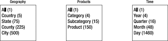
From these dimensions, we select the attributes we want included in aggregation designs. So we make selections based on what queries we think users will make, shown in Figure 13-20. For each of these combinations, Analysis Services will calculate the values for every combination of members. So for the All-All-All aggregation, it's simply a total of every measure value, resulting in one cell. Country-Subcategory-Year is 5×15×4 = 300 values, and City-Product-Day is 500×150×1460 = 109,500,000 values.

Figure 13.20. Selecting aggregations

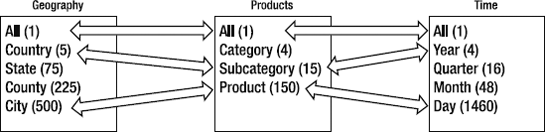
Once SSAS has these values cached, then results from queries simply use the largest aggregation possible, select the necessary members, and do the math. For example, if a user wants to see data from each year for sales of Road Bikes in France, SSAS can use the Country-Subcategory-Year aggregation, select the values for Road Bikes in France, and return them. If the user made the same query, but for the Bicycles category, Analysis Services could use the same aggregation, select out the values for each of the subcategories under Bicycle, add them, and return them.

However, if a user wants to see a breakdown of Road Bike sales by Year for each of the states in the United States, SSAS cannot use the Country-Subcategory-Year aggregation, as there is no way to get to the values for each state. So it drops down to the leaf-level aggregation of City-Product-Day, queries out the values for the Road Bike sales in the United States, and performs the calculations necessary to get to a breakdown by State, Subcategory, and Year. The amount of math necessary here indicates this is going to be a longer-running query...

So aggregation design is a trade-off between the space necessary in the file system to pre-cache the aggregation values and query time. If we had tons of space and lots of time to process a cube, it seems like it would make sense to just create aggregations for every possible combination of attributes. However, when you start considering the Cartesian products of all the attribute relationships in your cube, you can see that "tons of space" quickly becomes unrealistic. So aggregation design is a trade-off between storage space/processing time and query performance.

Creating an Aggregation

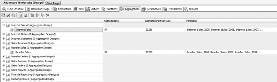
Aggregations for a cube are managed on the Aggregations tab of the cube designer in BIDS, as shown in Figure 13-21. Under each measure group are listed the aggregation designs for that group. For a given measure group, you can create multiple aggregation designs, then assign the aggregation designs to various partitions. An aggregation design will contain multiple aggregations.

Figure 13.21. The aggregation designer in BIDS

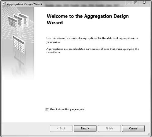
To create a new aggregation design, right-click on the measure group and select Design Aggregations to open the Aggregation Design Wizard (Figure 13-22). The wizard will allow you to select one or more partitions and create an aggregation design for them. One reason you may want a different aggregation design for a given partition is that it is loaded under different usage scenarios. For example, take the partition design scheme we talked about earlier—partitioning the data by year. Odds are that there will be far more queries against the current year's data than previous years', so the current year partition will probably have different aggregation usage.

Figure 13.22. The Aggregation Design Wizard

Once you've selected one or more partitions, then the wizard will ask you to select the attributes for each dimension to be included in the aggregation design, as shown in Figure 13-23. These settings guide the aggregation designer as to whether to include an attribute when calculating aggregations.

Figure 13.23. Selecting measures for the aggregation wizard

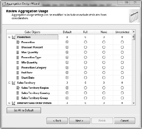
Each of these options indicates how the dimension attribute should be used in calculating aggregations. There's a list of all the dimensions in the cube, and each of the attributes in each dimension. For each attribute you indicate whether it should be included in every aggregation (Full), no aggregation (None), or "it depends" (Default or Unrestricted). Unrestricted means that you are allowing the aggregation designer to perform a cost/benefit analysis on the attribute and evaluate if it is a good candidate for an aggregation design. Attributes you anticipate to be queried often should be set to Unrestricted, while attributes you don't anticipate being queried often should be set to None.

Default implements a more complex rule depending on the attribute. The granularity attribute will be treated as unrestricted (perform cost/benefit analysis and include if suitable). All attributes that are in a natural hierarchy (1:n relationships from the top down) are considered as candidates for aggregation. Any other attribute is not considered for aggregation.

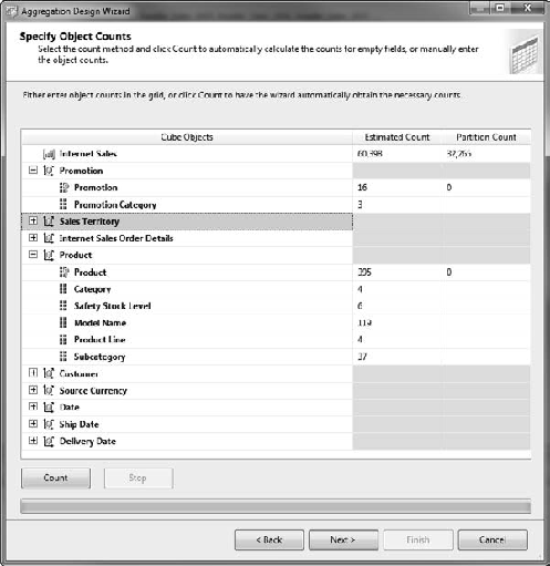
The next page in the wizard displays the counts for the measure group you're working on, as well as the attributes for all the dimensions included, as shown in Figure 13-24. You can have the wizard run a count of the current objects, or you can enter your own values if you are designing for a different scenario than what's currently defined.

Figure 13.24. Specifying the object counts in the database

The next page of the wizard, shown in Figure 13-25, is the heart of the aggregation designer. Here you select how you want the designer to proceed. You can set a maximum storage (in MB or GB), a specific performance gain (estimated), or a "keep running until I click Stop" to design the aggregations. Once you select the option, click the Start button to start the designer running. You'll see a chart generating something similar to what's shown in the example. The x axis is the size of the aggregation storage, the y axis is the aggregation optimization level in percent.

Figure 13.25. The aggregation options page of the Aggregation Design Wizard

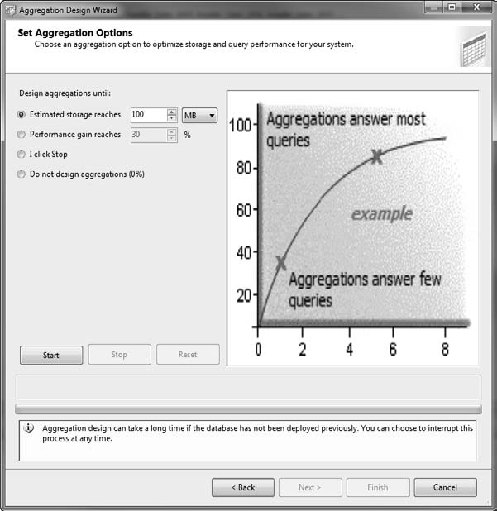
Once the designer stops (or you stop it), you'll get a result regarding the number of aggregations designed and the optimization level. Then you can either change the settings and run it again, or click the Next button. The final page of the wizard allows you to name the Aggregation design and either save the design or deploy it and process it immediately (probably not a great idea to do in production in the middle of the workday).

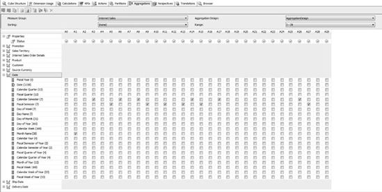
Once you've completed this wizard, Analysis Services will have the initial aggregation design set for the partitions you've set up. If you want to see the results of the aggregation design, click the "Advanced View" button in the toolbar. The aggregation viewer will show which attributes were included for each aggregation, as shown in Figure 13-26. Once you select the measure group and aggregation design at the top, you'll get a grid showing a column for each aggregation, and a checked box for each dimension attribute included in the aggregation.

Figure 13.26. Advanced aggregation design view

The grid of checked boxes in Figure 13-26 is a "first best guess" by SSAS, based on a cold, clean look at the cube design. The next step is to see how the aggregation design fares once it's been tested under load. For this SSAS has a Usage Based Optimization Wizard, or UBO. The UBO will look at the query records for the partitions covered by an aggregation design and evaluate how the aggregations perform based on what queries users are actually running.

Preparing an Aggregation for Use

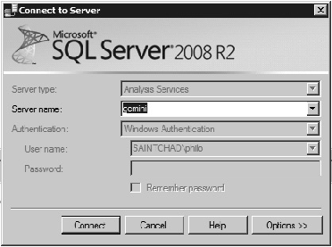
The first step to prepare for using the UBO is to enable the query log for SSAS. Analysis Services can run a query log to track the performance of every user query against a server. The query log is disabled by default (so unsuspecting admins don't have databases being filled up by query logs). To enable the query log, open SQL Server Management Studio and connect to the Analysis Services Server, as shown in Figure 13-27.

Figure 13.27. Connecting SSMS to an Analysis Server

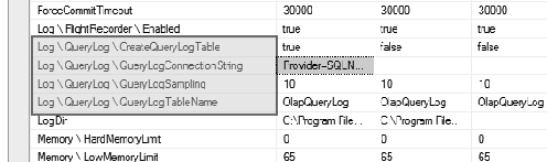
Once you've connected, open the properties dialog for the server by right-clicking the server name and selecting Properties. In the Properties dialog, you're interested in the Log QueryLog settings. Set the QueryLogConnectionString property to connect to a SQL Server instance. The QueryLogTableName value will be the name of the log table. You can connect to an existing table (which will have to have the appropriate schema), or by setting the CreateQueryLogTable setting to True, as shown in Figure 13-28.

Figure 13.28. Setting server properties for query logging

After running the query logs for a while, you'll be able to run the usage-based optimization wizard. You run the wizard by right-clicking on an aggregation design and selecting "Usage Based Optimization." From this point the wizard is just like the aggregation design wizard; however, behind the scenes, in addition to evaluating the cube architecture, it is reviewing the query logs. Based on the query logs and the architecture, the UBO wizard will redesign the aggregation design optimization for the indicated usage.

Note

If you haven't configured the QueryLog for the SSAS server, the UBO wizard will notify you and fail out.

Once you've established the aggregation designs and are in production, you can still run the UBO wizard periodically to review aggregation designs against cube usage, and update the designs if necessary.

Scalability in Analysis Services depends on which kind of scaling you need to do: large numbers of end users, or large data sizes (or both). In general, the choices of how to scale are either scale up, meaning add additional processors, move to a more powerful CPU speed, or add more RAM; or you can scale out, referring to adding additional servers in parallel. Each method has benefits and drawbacks, and which direction to go also depends on the reason you need to scale.

Large Number of Users

First and foremost, if you have a large number of users on an Analysis Services cube, scale out to additional servers. There are a number of architectures possible—scaling out partitions, separating query servers and processing servers, using multiple query servers for load balancing and redundancy, and so on. The architecture in Figure 13-29 provides a load-balanced queue of Query Servers that query against a read-only cube loaded on a SAN.

Figure 13.29. Notional scale-out architecture for scalable user base

The database is loaded and processed on a processing server; then the processed database is detached, copied to the shared SAN drive, and attached to the instance there. Since the database is read-only, no editing or writeback is possible. However, current writeback scenarios are generally much smaller-scale so you shouldn't need this approach.

Tip

If you want to load-test your Analysis Services Server without having a thousand users try it and break it, check out the ASLoadSim package at http://www.codeplex.com/SQLSrvAnalysisSrvcs, which includes code for running load tests as well as a document on SSAS Load Testing Best Practices.

Until recently, Microsoft strongly discouraged running SQL Server in a virtual environment, simply because enterprise databases and database applications generally get dedicated servers on their own. So virtualizing a database server and taking the virtualization hit didn't seem to make sense.

However, with the growth of adoption of SQL Server's BI platforms (often necessitating additional dedicated servers that aren't as heavily loaded), and improvements in Hyper-V performance and integration (load testing shows a SQL Server in a Hyper-V environment takes only about a 5% hit on performance), Microsoft now supports SQL Server in a virtualized environment.

Additionally, while the new Resource Governor in the SQL Server Relational Database gives DBAs finer control over services located on the same server, there is no similar feature for the BI services. So Microsoft now recommends setting up a BI environment (Integration Services, Analysis Services, Reporting Services) in dedicated virtual servers on a single physical server. Then the individual servers can be throttled by the Hyper-V infrastructure.

Finally, a tiny note about licensing—SQL Server Enterprise Edition has an interesting quirk in the per-processor licensing. If you license all the physical processors on a server, then any SQL Server instance you install on the virtual guest servers is also covered. So, if you need a number of independent but lightly-loaded SQL Servers, you could buy a host server with two quad-processor CPUs, then put eight guest machines on Hyper-V, each with a dedicated CPU core. Buy two SQL Server Enterprise Edition processor licenses for the two physical procs, and all of the guest SQL Server instances are licensed as well.

Since PowerPivot enables users to consume data from various sources, publish them to SharePoint, and refresh data periodically, there is a unique administrative challenge in that users may create PowerPivot reports that put excessive burdens on their servers. It's also possible that a PowerPivot report created on an ad-hoc basis turns out to be very popular, and a large number of people are running it on a regular basis, putting an extreme load on the PowerPivot server.

Given the potential for users to create significant loads on business intelligence and collaboration servers, it's very important to be able to track what's going on, and why, in the PowerPivot sandbox on your servers. With that in mind, the product group has added a management dashboard to the PowerPivot add-in for SharePoint 2010. To get to the management dashboard, open the SharePoint 2010 Central Administration application (Start

Figure 13.30. The PowerPivot management dashboard in SharePoint 2010

The SharePoint management dashboard provides a very useful perspective on the PowerPivot deployment from two aspects. First, you can easily identify PowerPivot workbooks that are putting a severe load on your server. Then you can analyze how heavily used that workbook is. For workbooks that are lightly used but loading the server and data sources, you may just want to contact the author and see if he or she can filter some of the data that's being loaded or take other steps to reduce the load.

The infrastructure charts at the top show Average Instance CPU, Memory, and Query Response Times. (The page is a standard SharePoint web part page, so you can add additional web parts and reports if you desire.) There are reports for Workbook Activity, Data Refresh Activity, and Data Refresh Failures.

The Workbook Activity Chart, shown in Figure 13-31, is a very useful chart. It's a bubble chart that helps to show the most active workbooks. The y axis is the number of users, while the x axis is the number of queries, and the size of the bubble is the size of the workbook. So we can interpret the bubbles—a large bubble that is low but to the far right is a large quantity of data that is heavily used by a small user base. On the other hand, a large bubble that is higher on the y axis is used by more people. Even if it's not as large and not as heavily used, it may be higher priority for IT review and possibly redesign.

Figure 13.31. The Workbook Activity Chart

Workbooks that are used by a lot of analysts, however, create a different problem. Given the ad-hoc nature of PowerPivot workbooks, the loading may simply be a result of heavy usage. In that case, you will probably want to evaluate having the PowerPivot data reengineered into a formal SSAS cube that can be optimized with consideration of the techniques and practices outlined in this chapter and elsewhere. As noted in Chapter 12, there is no "built-in" way to migrate a PowerPivot cube to SQL Server Analysis Services, so the workbook will have to be rebuilt following the guidance in the workbook.