
APPENDIX A
![]()
Choosing proper datatypes to match the domain chosen in logical modeling is an important task. One datatype might be more efficient than another of a similar type. For example, you can store integer data in an integer datatype, a numeric datatype, a floating point datatype, a character type, or even a binary column, but these datatypes certainly aren’t alike in implementation or performance.
In this appendix, I’ll introduce you to all the intrinsic datatypes that Microsoft provides and discuss the situations where they’re best used. The following is a list of the datatypes I’ll cover. I’ll discuss when to use them and in some cases why not to use them.
- bit: Stores either 1, 0, or NULL. Used for Boolean-type columns.
- tinyint: Non-negative values between 0 and 255.
- smallint: Integers between -32,768 and 32,767.
- int: Integers between 2,147,483,648 and 2,147,483,647 (-2 31 to 2 31 – 1).
- bigint: Integers between 9,223,372,036,854,775,808 and 9,223,372,036,854,775,807 (that is, -2 63 to 2 63 – 1) .
- decimal: Values between -10 38 + 1 through 10 38 – 1.
- money: Values from -922,337,203,685,477.5808 through 922,337,203,685,477.5807.
- smallmoney: Values from -214,748.3648 through + 214,748.3647.
- Approximate numeric data: Stores approximations of numbers. Provides for a large range of values.
- float (N): Values in the range from -1.79E + 308 through 1.79E + 308.
- real: Values in the range from -3.40E + 38 through 3.40E + 38. real is a synonym for a float(24) datatype.
- Date and time: Stores date values, including time of day.
- date: Date-only values from January 1, 0001 to December 31, 9999 (3 bytes).
- time: Time of day–only values to 100 nanoseconds (3–5 bytes). Note that the range of this type is from 0:00 to 23:59:59 and some fraction of a second based on the precision you select.
- datetime2: Despite the hideous name, this type will store dates from January 1, 0001 to December 31, 9999, to 100-nanosecond accuracy (6–8 bytes). The accuracy is based on the precision you select.
- datetimeoffset: Same as datetime2 but includes an offset from UTC time (8–10 bytes).
- smalldatetime: Dates from January 1, 1900 through June 6, 2079, with accuracy to 1 minute (4 bytes). (Note: it is suggested to phase out usage of this type and use the more standards-oriented datetime2, though smalldatetime is not technically deprecated.)
- datetime: Dates from January 1, 1753 to December 31, 9999, with accuracy to ∼3 milliseconds (stored in increments of .000, .003, or .007 seconds) (8 bytes). (Note: it is suggested to phase out usage of this type and use the more standards-oriented datetime2, though datetime is not technically deprecated)
- Character (or string) data: Used to store textual data, such as names, descriptions, notes, and so on.
- char: Fixed-length character data up to 8,000 characters long.
- varchar: Variable-length character data up to 8,000 characters long.
- varchar(max): Large variable-length character data; maximum length of 231 – 1 (2,147,483,647) bytes, or 2 GB.
- text: Large text values; maximum length of 231 – 1 (2,147,483,647) bytes, or 2 GB. (Note that this datatype is outdated and should be phased out in favor of the varchar(max) datatype.)
- nchar, nvarchar, ntext: Unicode equivalents of char, varchar, and text (with the same deprecation warning for ntext as for text).
- Binary data: Data stored in bytes, rather than as human-readable values, for example, files or images.
- binary: Fixed-length binary data up to 8,000 bytes long.
- varbinary: Variable-length binary data up to 8,000 bytes long.
- varbinary(max): Large binary data; maximum length of 231 – 1 (2,147,483,647) bytes, or 2 GB.
- image: Large binary data; maximum length of 231 – 1 (2,147,483,647) bytes, or 2 GB. (Note that this datatype is outdated and should be phased out for the varbinary(max) datatype.)
- Other scalar datatypes: Datatypes that don’t fit into any other groups nicely, but are still interesting.
- rowversion (or timestamp): Used for optimistic locking.
- uniqueidentifier: Stores a globally unique identifier (GUID) value.
- cursor: Datatype used to store a cursor reference in a variable. Cannot be used as a column in a table.
- table: Used to hold a reference to a local temporary table. Cannot be used as a column in a table.
- sql_variant: Stores data of most any datatype.
- Not simply scalar: For completeness, I mention these types, but they are not covered in any detail. These types are XML, hierarchyId, and the spatial types (geometry and geography). hierarchyId is used in Chapter 8 when dealing with hierarchical data patterns.
Although we’ll look at all these datatypes, this doesn’t mean you’ll have a need for all of them. Choosing a datatype needs to be a specific task to meet the needs of the client with the proper datatype. You could just store everything in unlimited-length character strings (this was how some systems worked in the old days), but this is clearly not optimal. From the list, you’ll choose the best datatype, and if you cannot find one good enough, you can use the CLR and implement your own. The proper datatype choice is the first step in making sure the proper data is stored for a column.
![]() Note I include information in each section about how the types are affected by using compression. This information refers to row-level compression only. For page-level compression information, see Chapter 10. Also note that compression is available only in the Enterprise Edition of SQL Server 2008 (and later).
Note I include information in each section about how the types are affected by using compression. This information refers to row-level compression only. For page-level compression information, see Chapter 10. Also note that compression is available only in the Enterprise Edition of SQL Server 2008 (and later).
Precise Numeric Data
You can store numerical data in many base datatypes, depending upon the actual need you are trying to fill. There are two different classes of numeric data: precise and approximate. The differences are important and must be well understood by any architect who’s building a system that stores readings, measurements, or other numeric data.
Precise values have no error in the way they’re stored, from integer to floating point values, because they have a fixed number of digits before and after the decimal point (or radix).
Approximate datatypes don’t always store exactly what you expect them to store. However, they are useful for scientific and other applications where the range of values varies greatly.
The precise numeric values include the bit, int, bigint, smallint, tinyint, decimal, and money datatypes (money and smallmoney). I’ll break these down again into three additional subsections: whole numbers and fractional numbers. This is done so we can isolate some of the discussion down to the values that allow fractional parts to be stored, because quite a few mathematical “quirks” need to be understood surrounding using those datatypes. I’ll mention a few of these quirks, most importantly with the money datatypes. However, when you do any math with computers, you must be careful how rounding is achieved and how this affects your results.
Integer Values
Whole numbers are, for the most part, integers stored using base-2 values. You can do bitwise operations on them, though generally it’s frowned upon in SQL. Math performed with integers is generally fast because the CPU can perform it directly using registers. I’ll cover five integer sizes: tinyint, smallint, int, and bigint.
The biggest thing that gets a lot of people is math with integers. Intuitively, when you see an expression like:
SELECT 1/2;
You will immediately expect that the answer is .5. However, this is not the case because integers don’t work this way; integer math only return integer values. The next intuitive leap you will probably make is that .5 should round up to 1, right? Nope, even the following query:
SELECT CAST(.99999999 AS integer);
returns 0. Instead of rounding, integer math truncates values, because it performs math like you did back in elementary school. For example, consider the following equation, 305, divided by 100:
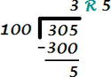
In a query, you get the whole number result using the division operator, and to get the remainder, you use the modulo operator (%). So you could execute the following query to get the division answer and the remainder:
SELECT 305 / 100, 305 % 100;
This returns 3 and 5. (The modulo operator is a very useful operator indeed.) If you want the result to be a non-whole number you need to cast at least one of the values to a datatype with a fractional element, like numeric, either by using cast, or a common method is to cast one of the factors to numeric, or by simply multiplying the first factor by 1.0:
SELECT CAST(305 as numeric)/ 100, (305 * 1.0) / 100;
These mathematical expressions now both return 3.050000, which is the value that the user is most likely desiring to get, much like the person dividing 1 by 2 expects to get .5.
tinyint
- Domain: Non-negative whole numbers from 0 through 255.
- Storage: 1 byte.
- Discussion:
- tinyints are used to store small non-negative integer values. When using a single byte for storage, if the values you’ll be dealing with are guaranteed always to be in this range, a tinyint is perfect. A great use for this is for the primary key of a domain table that can be guaranteed to have only a couple values. The tinyint datatype is especially useful in a data warehouse to keep the surrogate keys small. However, you have to make sure that there will never be more than 256 values, so unless the need for performance is incredibly great (such as if the key will migrate to tables with billions and billions of rows), it’s best to use a larger datatype.
- Row Compression Effect:
- No effect, because 1 byte is the minimum for the integer types other than bit.
smallint
- Domain: Whole numbers from -32,768 through 32,767 (or -2 15 through 2 15 – 1).
- Storage: 2 bytes.
- Discussion:
- If you can be guaranteed to need values only in this range, the smallint can be a useful type. It requires 2 bytes of storage.
- One use of a smallint that crops up from time to time is as a Boolean. This is because, in earlier versions of Visual Basic, 0 equaled False and -1 equaled True (technically, VB would treat any nonzero value as True, but it used -1 for its representation of False). Storing data in this manner is not only a tremendous waste of space—2 bytes versus potentially 1/8th of a byte for a bit, or even a single byte for a char(1)—'Y' or 'N'. It’s also confusing to all the other SQL Server programmers. ODBC and OLE DB drivers do this translation for you, but even if they didn’t, it’s worth the time to write a method or a function in VB to translate True to a value of 1.
- Row Compression Effect:
- The value will be stored in the smallest number of bytes required to represent the value. For example, if the value is 10, it would fit in a single byte; then it would use 1 byte, and so forth, up to 2 bytes.
int
- Domain: Whole numbers from -2,147,483,648 to 2,147,483,647 (that is, –2 31 to 2 31 – 1).
- Storage: 4 bytes.
- Discussion:
- The integer datatype is frequently employed as a primary key for tables, because it’s small (it requires 4 bytes of storage) and efficient to store and retrieve.
- One downfall of the int datatype is that it doesn’t include an unsigned version, which for a 32-bit version could store non-negative values from 0 to 4,294,967,296 (2 32). Because most primary key values start out at 1, this would give you more than 2 billion extra values for a primary key value without having to involve negative numbers that can be confusing to the user. This might seem unnecessary, but systems that have billions of rows are becoming more and more common.
- An application where the storage of the int column plays an important part is the storage of IP addresses as integers. An IP address is simply a 32-bit integer broken down into four octets. For example, if you had an IP address of 234.23.45.123, you would take (234 * 2 3) + (23 * 22) + (45 * 21) + (123 * 20). This value fits nicely into an unsigned 32-bit integer, but not into a signed one. However, the 64-bit integer (bigint, which is covered next) in SQL Server covers the current IP address standard nicely but requires twice as much storage. Of course, bigint will fall down in the same manner when we get to IPv6 (the forthcoming Internet addressing protocol), because it uses a full 64-bit unsigned integer.
- Row Compression Effect:
- The value will be stored in the smallest number of bytes required to represent the value. For example, if the value is 10, it would fit in a single byte; then it would use 1 byte, and so forth, up to 4 bytes.
bigint
- Domain: Whole numbers from -9,223,372,036,854,775,808 to 9,223,372,036,854,775,807 (that is, –2 63 to 2 63 – 1).
- Storage: 8 bytes.
- Discussion:
- One of the common reasons to use the 64-bit datatype is as a primary key for tables where you’ll have more than 2 billion rows, or if the situation directly dictates it, such as the IP address situation I previously discussed. Of course, there are some companies where a billion isn’t really a very large number of things to store or count, so using a bigint will be commonplace to them. As usual, the important thing is to size your utilization of any type to the situation, not using too small or even too large of a type than is necessary.
- Row Compression Effect:
- The value will be stored in the smallest number of bytes required to represent the value. For example, if the value is 10, it would fit in a single byte; then it would use 1 byte, and so forth, up to 8 bytes.
Decimal Values
The decimal datatype is precise, in that whatever value you store, you can always retrieve it from the table. However, when you must store fractional values in precise datatypes, you pay a performance and storage cost in the way they’re stored and dealt with. The reason for this is that you have to perform math with the precise decimal values using SQL Server engine code. On the other hand, math with IEEE floating point values (the float and real datatypes) can use the floating point unit (FPU), which is part of the core processor in all modern computers. This isn’t to say that the decimal type is slow, per se, but if you’re dealing with data that doesn’t require the perfect precision of the decimal type, use the float datatype. I’ll discuss the float and real datatypes more in the “Approximate Numeric Data” section.
decimal (alias: numeric)
- Domain: All numeric data (including fractional parts) between –10 38 + 1 through 10 38 – 1.
- Storage: Based on precision (the number of significant digits): 1–9 digits, 5 bytes; 10–19 digits, 9 bytes; 20–28 digits, 13 bytes; and 29–38 digits, 17 bytes.
- Discussion:
- The decimal datatype is a precise datatype because it’s stored in a manner that’s like character data (as if the data had only 12 characters, 0 to 9 and the minus and decimal point symbols). The way it’s stored prevents the kind of imprecision you’ll see with the float and real datatypes a bit later. However, decimal does incur an additional cost in getting and doing math on the values, because there’s no hardware to do the mathematics.
- To specify a decimal number, you need to define the precision and the scale:
- Precision is the total number of significant digits in the number. For example, 10 would need a precision of 2, and 43.00000004 would need a precision of 10. The precision may be as small as 1 or as large as 38.
- Scale is the possible number of significant digits to the right of the decimal point. Reusing the previous example, 10 would require a scale of 0, and 43.00000004 would need 8.
- Numeric datatypes are bound by this precision and scale to define how large the data is. For example, take the following declaration of a numeric variable:
DECLARE @testvar decimal(3,1)
- This allows you to enter any numeric values greater than -99.94 and less than 99.94. Entering 99.949999 works, but entering 99.95 doesn’t, because it’s rounded up to 100.0, which can’t be displayed by decimal(3,1). Take the following, for example:
SELECT @testvar = -10.155555555;
SELECT @testvar;
- This returns the following result:
-------------------
-10.2
- This rounding behavior is both a blessing and a curse. You must be careful when butting up to the edge of the datatype’s allowable values. There is a setting—SET NUMERIC_ROUNDABORT ON— that causes an error to be generated when a loss of precision would occur from an implicit data conversion. That’s kind of like what happens when you try to put too many characters into a character value.
- Take the following code:
SET NUMERIC_ROUNDABORT ON;
DECLARE @testvar decimal(3,1);
SELECT @testvar = -10.155555555;
SET NUMERIC_ROUNDABORT OFF;--this setting persists for a connection
- This causes the following error:
Msg 8115, Level 16, State 7, Line 3
Arithmetic overflow error converting numeric to data type numeric.
- SET NUMERIC_ROUNDABORT can be quite dangerous to use and might throw off applications using SQL Server if set to ON. However, if you need guaranteed prevention of implicit round-off due to system constraints, it’s there.
As far as usage is concerned, you should generally use the decimal datatype as sparingly as possible, and I don’t mean this negatively. There’s nothing wrong with the type at all, but it does take that little bit more processing than integers or real data, and hence there’s a performance hit. You should use it when you have specific values that you want to store where you can’t accept any loss of precision. Again, I’ll deal with the topic of loss of precision in more detail in the section “Approximate Numeric Data.” The decimal type is commonly used as a replacement for the money type, because it has certain round-off issues that decimal does not.
- Row Compression Effect:
- The value will be stored in the smallest number of bytes that are necessary to provide the precision necessary, plus 2 bytes overhead per row. For example, if you are storing the value of 2 in a numeric(28,2) column, it needn’t use all the possible space; it can use the space of a numeric(3,2), plus the 2 bytes overhead.
Money Types
There are two intrinsic datatypes that are for storing monetary values. Both are based on integer types, with a fixed four decimal places. These types are as follows:
- money
- Domain: -922,337,203,685,477.5808 to 922,337,203,685,477.5807
- Storage: 8 bytes
- smallmoney
- Domain: -214,748.3648 to 214,748.3647
- Storage: 4 bytes
The money datatypes are generally considered a poor choice of datatype, even for storing monetary values, because they have a few inconsistencies that can cause a good deal of confusion. First, you can specify units, such as $ or £, but the units are of no real value. For example:
CREATE TABLE dbo.testMoney
(
moneyValue money
);
go
INSERT INTO dbo.testMoney
VALUES ($100);
INSERT INTO dbo.testMoney
VALUES (100);
INSERT INTO dbo.testMoney
VALUES (£100);
GO
SELECT * FROM dbo.testMoney;
The query at the end of this code example returns the following results (each having the exact same value.):
moneyValue
----------
100.00
100.00
100.00
The second problem is that the money datatypes have well-known rounding issues with math. I mentioned that these types are based on integers (the range for smallmoney is -214,748.3648 to 214,748.3647, and the range for an integer is 2,147,483,648 to 2,147,483,647). Unfortunately, as I will demonstrate, intermediate results are stored in the same types, causing unexpected rounding errors. For example:
DECLARE @money1 money = 1.00,
@money2 money = 800.00;
SELECT CAST(@money1/@money2 as money);
This returns the following result:
---------------------
0.0012
However, try the following code:
DECLARE @decimal1 decimal(19,4) = 1.00,
, @decimal2 decimal(19,4) = 800.00;
SELECT CAST(@decimal1/@decimal2 as decimal(19,4));
It returns the following result:
----------------
0.0013
Why? Because money uses only four decimal places for intermediate results, where decimal uses a much larger precision:
SELECT @money1/@money2;
SELECT @decimal1/@decimal2;
This code returns the following results:
---------------------
0.0012
---------------------------------------
0.0012500000000000000
That’s why there are round-off issues. And if you turned SET NUMERIC_ROUNDABORT ON, the decimal example would fail, telling you that you were losing precision, whereas there is no way to stop the roundoff from occurring with the money types. The common consensus among database architects is to avoid the money datatype and use a numeric type instead, because of the following reasons:
- Numeric types give the answers to math problems in the natural manner that’s expected.
- Numeric types have no built-in units to confuse matters.
Even in the previous version of SQL Server, the following statement was included in the monetary data section: “If a greater number of decimal places are required, use the decimal datatype instead.” Using a decimal type instead gives you the precision needed. To replicate the range for money, use DECIMAL(19,4), or for smallmoney, use DECIMAL(10,4). However, you needn’t use such large values if you don’t need them. If you happen to be calculating the national debt or my yearly gadget allowance, you might need to use a larger value.
- Row Compression Effect:
- The money types are simply integer types with their decimal places shifted. As such, they are compressed in the same manner that integer types would be. However, since the values would be larger than they appear (because of the value 10 being stored as 10.000, or 10000 in the physical storage), the compression would be less than for an integer of the same magnitude.
Approximate numeric values contain a decimal point and are stored in a format that’s fast to manipulate. They are called floating point because they have a fixed number of significant digits, but the placement of the decimal point “floats,” allowing for really small numbers or really large numbers. Approximate numeric values have some important advantages, as you’ll see later in this appendix.
Approximate is such a negative term, but it’s technically the proper term. It refers to the real and float datatypes, which are IEEE 75454 standard single- and double-precision floating point values. The number is stored as a 32-bit or 64-bit value, with four parts:
- Sign: Determines whether this is a positive or negative value.
- Exponent: The exponent in base-2 of the mantissa.
- Mantissa: Stores the actual number that’s multiplied by the exponent (also known as the coefficient or significand).
- Bias: Determines whether the exponent is positive or negative.
A complete description of how these datatypes are formed is beyond the scope of this book but may be obtained from the IEEE body at www.ieee.org .
- float [ (N) ]
- Domain: –1.79E + 308 through 1.79E + 308. The float datatype allows you to specify a certain number of bits to use in the mantissa, from 1 to 53. You specify this number of bits with the value in N. The default is 53.
- Storage: See Table A-1
Table A-1. Floating Point Precision and Storage Requirements
| N (Number of Mantissa Bits for Float) | Precision | Storage Size |
|---|---|---|
| 1–24 | 7 | 4 bytes |
| 25–53 | 15 | 8 bytes |
- real
- real is a synonym for float(24).
At this point, SQL Server rounds all values of N up to either 24 or 53. This is the reason that the storage and precision are the same for each of the values.
- Discussion:
- Using these datatypes, you can represent most values from -1.79E + 308 to 1.79E + 308 with a maximum of 15 significant digits. This isn’t as many significant digits as the numeric datatypes can deal with, but the range is enormous and is plenty for almost any scientific application (The distance from the Earth to the Andromeda galaxy is only 2.5 * power(10,19) kilometers!), . These datatypes have a much larger range of values than any other datatype. This is because the decimal point isn’t fixed in the representation. In exact numeric types, you always have a pattern such as NNNNNNN.DDDD for numbers. You can’t store more digits than this to the left or right of the decimal point. However, with float values, you can have values that fit the following patterns (and much larger):
- 0.DDDDDDDDDDDDDDD
- NNNNN.DDDDDDDDDD
- 0.0000000000000000000000000000DDDDDDDDDDDDDDD
- NNNNNNNNNNNNNNN000000000000000000
- So, you have the ability to store tiny numbers, or large ones. This is important for scientific applications where you need to store and do math on an extreme range of values. The float datatypes are well suited for this usage.
- Row Compression Effect:
- The least significant bytes with all zeros are not stored. This is applicable mostly to non-fractional values in the mantissa.
Back in SQL Server 2005, the choice of datatype for storing date and time data was pretty simple. We had two datatypes for working with date and time values: datetime and smalldatetime. Both had a time element and a date element, and you could not separate them. Not having a simple date or time datatype was be a real bother at times because a rather large percentage of data only really needs the date portion.
In SQL Server 2008, a set of new datatypes were added that changed all of that. These were date, time, datetime2, and datetimeoffset. These new datatypes represent a leap of functionality in addition to the original datetime and smalldatetime. For the most part, the new types cover the range of date and time values that could be represented in the original types, though only the smalldatetime type can easily represent a point in time to the minute, rather than second. As of the 2012 release of SQL Server, the datetime and smalldatetime are suggested to be phased out for future use, and as such you should move work to datetime2 or one of the other date/time datatypes.
date
- Domain: Date-only values from January 1, 0001 to December 31, 9999.
- Storage: 3-byte integer, storing the offset from January 1, 0001.
- Accuracy: One day.
- Discussion:
- Of all the features added back in SQL Server in 2008, this one datatype was worth the price of the upgrade (especially since I don’t have to whip out my wallet and pay for it). The problem of how to store date values without time had plagued T-SQL programmers since the beginning of time (aka version 1.0).
-
With this type, you will be able to avoid the tricks you have needed to go through to ensure that date types had no time in order to store just a date value. In past versions of the book, I advocated the creation of your own pseudodate values stored in an integer value. That worked, but you could not use the built-in date functions without doing some “tricks.”
- Row Compression Effect:
- Technically you get the same compression as for any integer value, but dates in the “normal” range of dates require 3 bytes, meaning no compression is realized.
- Domain: Time of day only (note this is not a quantity of time, but a point in time on the clock).
- Storage: 3–5 bytes, depending on precision.
- Accuracy: To 100 nanoseconds, depending on how it is declared. time(0) is accurate to 1 second, time(1) to .1 seconds, up to time(7) as .0000001. The default is 100-nanosecond accuracy.
- Discussion:
- The time type is handy to have but generally less useful. Initially it will seem like a good idea to store a point in time, but in that case you will have to make sure that both times are for the same day. Rather, for the most part when you want to store a time value, it is a point in time, and you need one of the date + time types.
-
The time value can be useful for storing a time for a recurring activity, for example, where the time is for multiple days rather than a single point in time.
- Row Compression Effect:
- Technically you get the same compression as for any integer value, but time values generally use most of the bytes of the integer storage, so very little compression should be expected for time values.
- Domain: Dates from January 1, 0001 to December 31, 9999, with a time component.
- Storage: Between 6 and 8 bytes. The first 4 bytes are used to store the date, and the others an offset from midnight, depending on the accuracy.
- Accuracy: To 100 nanoseconds, depending on how it is declared. datetime(0) is accurate to 1 second, datetime(1) to .1 seconds, up to datetime(7) as .0000001. The default is 100-nanosecond accuracy.
- Discussion:
- This is a much better datatype than datetime. Technically, you get far better time support without being limited by the .003 accuracy issues that datetime is. The only downside I currently see is support for the type in your API.
-
What I see as the immediate benefit of this type is to fix the amount of accuracy that your users actually desire. Most of the time a user doesn’t desire fractional seconds, unless the purpose of the type is something scientific or technical. With datetime2, you can choose 1-second accuracy. Also, you can store .999 seconds, unlike datetime, which would round .999 up to 1, whereas .998 would round down to .997.
- Row Compression Effect:
- For the date portion of the type, dates before 2079 can save 1 byte of the 4 bytes for the date. Little compression should be expected for the time portion.
The datetimeoffset is the same as datetime2, but it includes an offset from UTC time (8–10 bytes).
- Domain: Dates from January 1, 0001 to December 31, 9999, with a time component. Includes the offset from the UTC time, in a format of [+|-] hh:mm. (Note that this is not time zone/daylight saving time aware. It simply stores the offset at the time of storage.)
- Storage: Between 8 and 10 bytes. The first 4 bytes are used to store the date, and just like datetime2, 2–4 will be used for the time, depending on the accuracy. The UTC offset is stored in the additional 2 bytes.
- Accuracy: To 100 nanoseconds, depending on how it is declared. datetimeoffset(0) is accurate to 1 second, datetimeoffset (1) to .1 seconds, up to datetimeoffset (7) as .0000001. The default is 100-nanosecond accuracy.
- Discussion:
- The offset seems quite useful but in many ways is more cumbersome than using two date columns, one for UTC and one for local (though this will save a bit of space). Its true value is that it defines an exact point in time better than the regular datetime type, since there is no ambiguity as to where the time was stored.
-
A useful operation is to translate the date from its local offset to UTC, like this:
DECLARE @LocalTime DateTimeOffset;
SET @LocalTime = SYSDATETIMEOFFSET();
SELECT @LocalTime;
SELECT SWITCHOFFSET(@LocalTime, ' + 00:00') As UTCTime;
- The true downside is that it stores an offset, not the time zone, so daylight saving time will still need to be handled manually.
- Row Compression Effect:
- For the date portion of the type, dates before 2079 can save 1 byte of the 4 bytes for the date. Little compression should be expected for the time portion.
- Domain: Date and time data values between January 1, 1900 and June 6, 2079.
- Storage: 4 bytes (two 2-byte integers: one for the day offset from January 1, 1900, the other for the number of minutes past midnight).
- Accuracy: One minute.
- Discussion:
- The smalldatetime datatype is accurate to 1 minute. It requires 4 bytes of storage. smalldatetime values are the best choice when you need to store the date and time of some event where accuracy of a minute isn’t a problem.
smalldatetime is suggested to be phased out of designs and replaced with datetime2, though it is very pervasive and will probably be around for several versions of SQL Server yet to come. Unlike datetime, there is not a direct replacement in terms of accuracy, as minimum datetime2 accuracy is to the second.
- Row Compression Effect:
- When there is no time stored, 2 bytes can be saved, and times less than 4 a.m. can save 1 byte.
- Domain: Date and time data values between January 1, 1753 and December 31, 9999.
- Storage: 8 bytes (two 4-byte integers: one for the day offset from January 1, 1753, and the other for the number of 3.33-millisecond periods past midnight).
- Accuracy: 3.33 milliseconds.
- Discussion:
- Using 8 bytes, datetime is a bit heavy on memory, but the biggest issue is regarding the precision. The biggest issue is that it is accurate to .003 seconds, leading to interesting roundoff issues. For example, very often a person will write an expression such as:
- WHERE datetimeValue < = '20110919 23:59:59.999'
- This is used to avoid getting any values for the next day of ‘20110920 00:00:00.000’. However, because of the precision, the expression
- SELECT CAST('20110919 23:59:59.999' AS datetime);
- Will return: 2011-09-20 00:00:00.000. Instead, you will need to use
- SELECT CAST('20110919 23:59:59.997' AS datetime);
- To get the max datetime value that is less than ‘20110920 00:00:00.000’
datetime is suggested to be phased out of designs and replaced with datetime2, though it is very pervasive and will probably be around for several versions of SQL Server yet to come.
- Row Compression Effect:
- For the date portion of the type, dates before 2079 can save 1 byte. For the time portion, 4 bytes are saved when there is no time saved, and it uses the first 2 bytes after the first 2 minutes and reaches the fourth byte after 4 a.m. After 4 a.m., compression can generally save 1 byte.
Discussion on All Date Types
Date types are often some of the most troublesome types for people to deal with. In this section, I’ll lightly address the following problem areas:
With the creation of new date and time (and datetime) types back in SQL Server 2008, there needed to be more functions to work with. Microsoft has added functions that return and modify dates and time with more precision than GETDATE or GETUTCDATE:
- SYSDATETIME: Returns system time to the nearest fraction of a second, with seven places of scale in the return value
- SYSDATETIMEOFFSET: Same as SYSDATETIME but returns the offset of the server in the return value
- SYSUTCDATETIME: Same as SYSDATETIME but returns the UTC date time rather than local time
- SWITCHOFFSET: Changes the offset for a datetimeoffset value
- TODATETIMEOFFSET: Converts a local date and time value to a given time zone
There have been a few changes to the basic date functions as well:
- DATENAME: Includes values for microsecond, nanosecond, and TZoffset. These will work differently for the different types. For example, TZoffset will work with datetime2 and datetimeoffset, but not the other types.
- DATEPART: Includes microsecond, nanosecond, TZoffset, and ISO_WEEK. ISO_WEEK is a feature that has been long desired by programmers who need to know the week of the year, rather than the nonstandard week value that SQL Server has previously provided.
- DATEADD: Supports micro and nanoseconds.
With all the date functions, you really have to be careful that you are cognizant of what you are requesting. For an example, how old is this person? Say you know that a person was born on December 31, 2008, and on January 3, 2009, you want to know their age. Common sense says to look for a function to take the difference between two dates. You are in luck—there is a DATEDIFF function. Executing the following:
DECLARE @time1 date = '20111231',
@time2 date = '20120102';
SELECT DATEDIFF(yy,@time1,@time2);
You see that the person is 0 years old right? Wrong! It returns 1.Ok, so if that is true, then the following should probably return 2, right?
DECLARE @time1 date = '20110101',
@time2 date = '20121231';
SELECT DATEDIFF(yy,@time1,@time2);
That also returns 1. So, no matter whether the date values are 1 day apart or 730, you get the same result? Yes, because the DATEDIFF function is fairly dumb in that it is taking the difference of the year value, not the difference in years. Then, to find out the age, you will need to use several functions.
So, what is the answer? We could do something fancier, likely by coming up with an algorithm based on the number of days, or months, or shifting dates to some common value, but that is way more like work than the really straightforward answer. Build a table of dates, commonly called a calendar (see Chapter 12).
This topic will probably seem really elementary, but the fact is that one of the largest blunders in the database implementation world is working with ranges of dates. The problem is that when you want to do inclusive ranges, you have always needed to consider the time in the equation. For example, the following criteria:
WHERE pointInTimeValue BETWEEN '2012-01-01' AND '2012-12-31'
means something different based on whether the values stored in pointInTimeValue have, or do not have, a time part stored. With the introduction of the date type, the need to worry about this issue of date ranges may eventually become a thing of the past, but it is still an issue that you’ll always need to worry about whether you need to worry about it.
The problem is that any value with the same date as the end value plus a time (such as '2012-12-31 12:00:00') does not fit within the preceding selecting criteria. Because you will miss all the activity that occurred on December 31 that wasn’t at midnight.
There are two ways to deal with this. Either code your WHERE clause like this:
WHERE pointInTimeValue > = '2012-01-01' and pointInTimeValue < '2013-01-01'
or use a calculated column to translate point-in-time values in your tables to date-only values (like dateValue as cast(pointInTimeValue as date)). Many times the date value will come in handy for grouping activity by day as well. Having done that, a value such as '2012-12-31 12:00:00' will be truncated to '2012-12-31 00:00:00', and a row containing that value will be picked up by selection criteria such as this:
WHERE pointInTimeValue BETWEEN '2012-01-01' AND '2012-12-31'
A common solution that I don’t generally suggest is to use a between range like this:
WHERE pointInTimeValue BETWEEN '2012-01-01' AND '2012-12-31 23:59:59.9999999'
The idea is that if the second value is less than the next day, values for the next day won’t be returned. The major problem with this solution has to do with the conversion of 23:59:59.9999999 to one of the various date datatypes. Each of the types will round up, so you must match the number of fractional parts to the precision of the type. For datetime2(3), you would need 23:59:59.999. If the pointInTimeValue column was of type: datetime, you would need use this:
WHERE pointInTimeValue BETWEEN '2009-01-01' AND '2009-12-31 23:59:59.997'
However, for a smalldatetime value, it would need to be this:
WHERE pointInTimeValue BETWEEN '2009-01-01' AND '2009-12-31 23:59'
and so on, for all of the different date types, which gets complicated by the new types where you can specify precision. I strongly suggest you avoid trying to use a maximum date value like this unless you are tremendously careful with the types of data and how their values round off.
For more information about how date and time data work with one another and converting from one type to another, read the topic “Using Date and Time Data” in Books Online.
Representing Dates in Text Formats
When working with date values in text, using a standard format is always best. There are many different formats used around the world for dates, most confusingly MMDDYYYY and DDMMYYYY (is 01022004 or 02012004 the same day, or a different day?). Although SQL Server uses the locale information on your server to decide how to interpret your date input, using one of the following formats ensures that SQL Server doesn’t mistake the input regardless of where the value is entered.
Generally speaking, it is best to stick with one of the standard date formats that are recognized regardless of where the user is. This prevents any issues when sharing data with international clients, or even with sharing it with others on the Web when looking for help.
There are several standards formats that will work:
- ANSI SQL Standard
- No time zone offset: 'YYYY-MM-DD HH:MM:SS'
- With time zone: 'YYYY-MM-DD HH:MM:SS –OH:OM' (Z, for Zulu, can be used to indicate the time zone is the base time of 00:00 offset, otherwise known as GMT [Greenwich Mean Time] or the most standard/modern name is UTC [Coordinated Universal Time].)
- ISO 8601
- Unseparated: 'YYYYMMDD'
- Numeric: 'YYYY-MM-DD'
- Time: 'HH:MM:SS.sssssss' (SS and .sssssss are optional)
- Date and time: 'YYYY-MM-DDTHH:MM:SS.sssssss'
- Date and time with offset: 'YYYY-MM-DDTHH:MM:SS.sssssss -OH:OM'
- ODBC
- Date: {d 'YYYY-MM-DD'}
- Time: {t 'HH:MM:SS'}
- Date and time: {ts 'YYYY-MM-DD HH:MM:SS'}
Using the ANSI SQL Standard or the ISO 8601 formats is generally considered the best practice for specifying date values. It will definitely feel odd when you first begin typing '2008-08-09' for a date value, but once you get used to it, it will feel natural.
The following are some examples using the ANSI and ISO formats:
SELECT CAST('2013-01-01' as date) AS dateOnly;
SELECT CAST('2013-01-01 14:23:00.003' AS datetime) as withTime;
You might also see values that are close to this format, such as the following:
SELECT CAST ('20130101' as date) AS dateOnly;
SELECT CAST('2013-01-01 T14:23:00.120' AS datetime) AS withTime;
For more information, check SQL Server 2012 Books Online under “Date and Time Format” Related to dates, a new function FORMAT has been added to SQL Server 2012 that will help you output dates in any format you need to. As a very brief example, consider the following code snippet:
DECLARE @DateValue datetime2(3) = '2012-05-21 15:45:01.456'
SELECT @DateValue as Unformatted,
FORMAT(@DateValue,'yyyyMMdd') as IsoUnseperated,
FORMAT(@DateValue,'yyyy-MM-ddThh:mm:ss') as IsoDateTime,
FORMAT(@DateValue,'D','en-US' ) as USRegional,
FORMAT(@DateValue,'D','en-GB' ) as GBRegional,
FORMAT(@DateValue,'D','fr-fr' ) as FRRegional;
This returns the following:
| Unformatted | IsoUnseperated | IsoDateTime |
| ----------------------- | -------------- | ------------------- |
| 2012-05-21 15:45:01.456 | 20120521 | 2012-05-21T03:45:01 |
|
USRegional |
GBRegional |
FRRegional |
| -------------------- | ----------- | ----------------- |
| Monday, May 21, 2012 | 21 May 2012 | lundi 21 mai 2012 |
The unformatted version is simply how it appears in SSMS using my settings. The IsoUnseperated value was built using a format mask of yyyyMMdd, and the IsoDateTime using a bit more interesting mask, each of which should be fairly obvious, but check the FORMAT topic in books online for a full rundown of features. The last two examples format the date in the manner of a given region, each of which could come in very handy building regionalized reports. Note that the Great Britain version doesn’t list the day of the week, whereas the United States and France do. FORMAT does more than just date data, but this is where we have generally felt the most pain with data through the years. so I mentioned it here.
There is another handy function PARSE that will let you take a value in a given regional version and parse information out of a formatted string. I won’t demonstrate PARSE, but rather wanted to make you aware of more tools to work with date data here in this date data section of the appendix.
Most data that’s stored in SQL Server uses character datatypes. In fact, usually far too much data is stored in character datatypes. Frequently, character columns are used to hold noncharacter data, such as numbers and dates. Although this might not be technically wrong, it isn’t ideal. For starters, storing a number with eight digits in a character string requires at least 8 bytes, but as an integer it requires 4 bytes. Searching on integers is far easier because 1 always precedes 2, whereas 11 comes before 2 in character strings. Additionally, integers are stored in a format that can be manipulated using intrinsic processor functions, as opposed to having SQL Server–specific functions deal with the data.
Domain: ASCII characters, up to 8,000 characters long.
Storage: 1 byte * length.
Discussion:
The char datatype is used for fixed-length character data. Every value will be stored with the same number of characters, up to a maximum of 8,000 bytes. Storage is exactly the number of bytes as per the column definition, regardless of actual data stored; any remaining space to the right of the last character of the data is padded with spaces. The default size if not specified is 1 (it is best practice to include the size).
You can see the possible characters by executing the following query:
SELECT number, CHAR(number)
FROM Tools.Number
WHERE number >=0 and number <= 255;
![]() Tip The numbers table is a common table that every database should have. It’s a table of integers that can be used for many utility purposes. In Chapter 12, I present a numbers table that you can use for this query.
Tip The numbers table is a common table that every database should have. It’s a table of integers that can be used for many utility purposes. In Chapter 12, I present a numbers table that you can use for this query.
- The maximum limit for a char is 8,000 bytes, but if you ever get within a mile of this limit for a fixed-width character value, you’re likely making a big design mistake because it’s extremely rare to have massive character strings of exactly the same length. You should employ the char datatype only in cases where you’re guaranteed to have exactly the same number of characters in every row.
- The char datatype is most often used for codes and identifiers, such as customer numbers or invoice numbers where the number includes alpha characters as well as integer data. An example is a vehicle identification number (VIN), which is stamped on most every vehicle produced around the world. Note that this is a composite attribute, because you can determine many things about the automobile from its VIN.
- Another example where a char column is usually found is in Social Security numbers (SSNs), which always have nine characters and two dashes embedded.
- Row Compression Effect:
- Instead of storing the padding characters, it removes them for storage and adds them back whenever the data is actually used.
![]() Note The setting ANSI_PADDING determines exactly how padding is handled. If this setting is ON, the table is as I’ve described; if not, data will be stored as I’ll discuss in the “varchar(length)” section. It’s best practice to leave this ANSI setting ON.
Note The setting ANSI_PADDING determines exactly how padding is handled. If this setting is ON, the table is as I’ve described; if not, data will be stored as I’ll discuss in the “varchar(length)” section. It’s best practice to leave this ANSI setting ON.
Domain: ASCII characters, up to 8,000 characters long.
Storage: 1 byte * length + 2 bytes (for overhead).
Discussion:
For the varchar datatype, you choose the maximum length of the data you want to store, up to 8,000 bytes. The varchar datatype is far more useful than char, because the data doesn’t have to be of the same length and SQL Server doesn’t pad out excess memory with spaces. There’s some reasonably minor overhead in storing variable-length data. First, it costs an additional 2 bytes per column. Second, it’s a bit more difficult to get to the data, because it isn’t always in the same location of the physical record. The default size if not specified is 1 (it is best practice to include the size).
Use the varchar datatype when your character data varies in length. The good thing about varchar columns is that, no matter how long you make the maximum, the space used by the column is based on the actual size of the characters being stored plus the few extra bytes that specify how long the data is.
ou’ll generally want to choose a maximum limit for your datatype that’s a reasonable value, large enough to handle most situations, but not too large as to be impractical to deal with in your applications and reports. For example, take people’s first names. These obviously require the varchar type, but how long should you allow the data to be? First names tend to be a maximum of 15 characters long, though you might want to specify 20 or 30 characters for the unlikely exception.
The most prevalent storage type for non-key values that you’ll use is varchar data, because, generally speaking, the size of the data is one of the most important factors in performance tuning. The smaller the amount of data, the less has to be read and written. This means less disk access, which is one of the two most important bottlenecks we have to deal with (networking speed is the other).
Row Compression Effect:
No effect.
Domain: ASCII characters, up to 231 – 1 characters (that is a maximum of 2 GB worth of text!).
Storage: There are a couple possibilities for storage based on the setting of the table option 'large value types out of row', which is set with the sp_tableoption system stored procedure:
- OFF =: The data for all the columns fits in a single row, and the data is stored in the row with the same storage costs for non-max varchar values. Once the data is too big to fit in a single row, data can be placed on more than one row. This is the default setting.
- ON =: You store varchar(max) values using 16-byte pointers to separate pages outside the table. Use this setting if the varchar(max) data will only seldom be used in queries.
Discussion:
The varchar(max) datatype is great replacement for the text datatype and all its quirks. You can deal with varchar(max) values using mostly the same functions and methods that you use with normal varchar values. There’s a minor difference, though. As the size of your varchar(max) column grows toward the upper boundary, it’s likely true that you aren’t going to want to be sending the entire value back and forth over the network most of the time. I know that even on my 100 MB LAN, sending 2 GB is no instantaneous operation, for sure.
There are a couple things to look at:
- The UPDATE statement has a .WRITE() clause to write chunks of data to the (max) datatypes. This is also true of varbinary(max).
- Unlike text and image values, (max) datatypes are accessible in AFTER triggers.
One word of warning for when your code mixes normal varchar and varchar(max) values in the same statement: normal varchar values do not automatically change datatype to a (max) type when the data being manipulated grows beyond 8,000 characters. For example, write a statement such as the following:
DECLARE @value varchar(max) = REPLICATE('X',8000) + REPLICATE('X',8000);
SELECT LEN(@value);
This returns the following result, which you would expect to be 16000, since you have two 8,000-character strings:
---------------
8000
The reason is that the type of the REPLICATE function is varchar, when replicating normal char values. Adding two varchar values together doesn’t result in a varchar(max) value. However, most of the functions return varchar(max) values when working with varchar(max) values. For example:
DECLARE @value varchar(max) = REPLICATE(cast('X' AS varchar(max)),16000);
SELECT LEN(@value);
This returns the following result:
----------------
16000
Row Compression Effect:
No effect.
Don’t use the text datatype for any reason in new designs. It might not exist in the next version of SQL Server (though I have written that statement for several versions of this book). Replace with varchar(max) whenever you possibly can. See SQL Server Books Online for more information.
Unicode Character Strings: nchar, nvarchar, nvarchar(max), ntext
Domain: ASCII characters, up to 215 – 1 characters (2 GB of storage).
Storage: Same as other character datatypes, though every character takes 2 bytes rather than 1. (Note there is no support for any of the variable-length Unicode storage.)
Discussion:
So far, the character datatypes we’ve been discussing have been for storing typical ASCII data. In SQL Server 7.0 (and NT 4.0), Microsoft implemented a new standard character format called Unicode. This specifies a 16-bit character format that can store characters beyond just the Latin character set. In ASCII—a 7-bit character system (with the 8 bits for Latin extensions)—you were limited to 256 distinct characters. This was fine for most English-speaking people but was insufficient for other languages. Asian languages have a character for each different syllable and are nonalphabetic; Middle Eastern languages use several different symbols for the same letter according to its position in the word. Unicode expanded the amount of characters and eliminated the need for code pages to allow for a vastly expanded character set (which allowed you to have multiple character sets in an 8-character encoding set in ASCII). SQL Server supports the Unicode Standard, version 3.2.
For these datatypes, you have the nchar, nvarchar, nvarchar(max), and ntext datatypes. They are the same as the similarly named types (without the n) that we’ve already described, except for one thing: Unicode uses double the number of bytes to store the information, so it takes twice the space, thus cutting by half the number of characters that can be stored.
One quick tip: if you want to specify a Unicode value in a string, you append an N (must be a capital N, a lowercase will give you an error) to the front of the string, like so:
SELECT N'Unicode Value';
![]() Tip You should migrate away from ntext as a datatype just as you should for the text datatype.
Tip You should migrate away from ntext as a datatype just as you should for the text datatype.
Row Compression Effect:
Just like their ASCII counterparts for fixed length types it will not store trailing blanks for the fixed-length types. As of SQL Server 2008R2, compression can compress Unicode values using what is known as the Standard Compression Scheme for Unicode (SCSU), which gives anywhere between 15 and 50 percent storage improvement depending on the character set. This is particularly interesting as a lot of third-party systems use Unicode storage “just in case,” and it is becoming more and more the norm to use Unicode for pretty much everything in a system to allow for the future, even if you never make use of anything other than a standard ASCII character.
Binary data allows you to store a string of bytes. It’s useful for storing just about anything, especially data from a client that might or might not fit into a character or numeric datatype. In SQL Server 2005, binary columns became even more useful, because you can use them when storing encrypted data. In Chapter 9, you’ll learn about the encryption capabilities of SQL Server.
One of the restrictions of binary datatypes is that they don’t support bitwise operators, which would allow you to do some powerful bitmask storage by being able to compare two binary columns to see not only whether they differ, but how they differ. The whole idea of the binary datatypes is that they store strings of bits. The bitwise operators can operate on integers, which are physically stored as bits. The reason for this inconsistency is fairly clear from the point of view of the internal query processor. The bitwise operations are operations that are handled in the processor, whereas the binary datatypes are SQL Server specific.
Binary literal values are specified as 0xB1B2B3 . . . BN. 0x tells you that it’s a hexadecimal value. B1 specifies the first single byte in hexadecimal.
Domain: Fixed-length binary data with a maximum length of 8,000 bytes.
Storage: Number of bytes the value is defined for. The default length is 1, if not specified (it is best practice to include a size).
Discussion:
The use of binary columns is fairly limited. You can use them to store any binary values that aren’t dealt with by SQL Server. Data stored in binary is simply a string of bytes:
DECLARE @value binary(10) = CAST('helloworld' AS binary(10));
SELECT @value;
This returns the following result:
----------------------
0x68656C6C6F776F726C64
Now you can reverse the process:
SELECT CAST(0x68656C6C6F776F726C64 AS varchar(10));
This returns the following result:
----------
helloworld
Note that casting the value HELLOWORLD gives you a different value:
----------------------
0x48454C4C4F574F524C44
This fact that these two binary values are different, even for textual data that would be considered equivalent on a case-insensitive collation, has been one use for the binary datatype: case-sensitive searches. This is generally not the best way to do a case sensitive comparison, as it’s far more efficient to use the COLLATE keyword and use a different collation if you want to do a case-insensitive comparison on string data.
Row Compression Effect:
Trailing zeros are not stored but are returned when the values are used.
Domain: Variable-length binary data with a maximum length of 8,000 bytes.
Storage: Number of bytes the value is defined for, plus 2 bytes for variable-length overhead. The default length is 1, if not specified (it is a best practice to include a size).
Discussion:
The usage is the same as binary, except the number of bytes is variable.
Row Compression Effect:
No effect.
Domain: Binary data, up to 231 – 1 bytes (up to 2 GB for storage) when data is stored in SQL Server files, up to the max of the storage for data stored in the filestream. For more information and examples about the filestream, check Chapter 7.
Storage: There are a couple possibilities for storage based on whether the data is stored using the filestream setting, as well as the setting of the table option 'large value types out of row':
- OFF =: If the data for all the columns fits in a single row, the data is stored in the row with the same storage costs for non-max varchar values. Once the data is too big to fit in a single row, data can be placed on greater than one row.
- ON =: You store varbinary(max) values using 16-byte pointers to separate pages outside the table. Use this setting if the varchar(max) data will only seldom be used in queries.
Discussion:
The varbinary(max) datatype provides the same kinds of benefits for large binary values as the varchar(max) does for text. Pretty much you can deal with varbinary(max) values using the same functions and the same methods as you do with the normal varbinary values.
What’s cool is that you can store text, JPEG and GIF images, and even Word documents and Excel spreadsheet data using the varbinary(max) type. On the other hand, it can be much slower and more programming work to use SQL Server as a storage mechanism for files, mostly because it’s slow to retrieve really large values from the database as compared to from the file system. You can, however, use a filestream access to get the best of both possible worlds by using Win32 access to a file in a directory within the context of a transaction. This approach is described in greater detail in Chapter 7.
Row Compression Effect:
No effect.
Just like the text datatype, the image datatype is being deprecated in this version of SQL Server. Don’t use the image datatype in new designs if at all possible. It very well may not exist in the next version of SQL Server. Replace with varbinary(max) in any location you can. See SQL Server Books Online for more information or if you have existing image column data that you need to manipulate.
Other Datatypes
The following datatypes are somewhat less easy to categorize but are still commonly employed in OLTP systems:
- bit
- rowversion (timestamp)
- uniqueidentifier
- cursor
- table
- sql_variant
Domain: 0, 1, or NULL.
Storage: A bit column requires 1 byte of storage per eight instances in a table. Hence, having eight bit columns will cause your table to be no larger than if your table had only a single bit column.
Discussion:
You use bit values as a kind of imitation Boolean value. A bit isn’t a Boolean value, in that it has values 0 and 1, not True and False. This is a minor distinction but one that needs to be made. You cannot execute code such as this:
IF (bitValue) DO SOMETHING;
A better term than a Boolean is a flag. A value of 1 means the flag has been set (such as a value that tells us that a customer does want e-mail promotions). Many programmers like to use character values 'yes' or 'no' for this, because this can be easier for viewing, but it can be harder to program with using built-in programming methods. In fact, the use of the bit datatype as a Boolean value has occurred primarily because many programming languages usually use 0 for False and nonzero for True (some use 1 or –1 explicitly).
You can index a bit column, but usually it isn’t of any value only to index it. Having only two distinct values in an index (technically three with NULL) makes for a poor index. (See Chapter 10 for more information about indexes. You may be able to use a filtered index to make some indexes on bit columns useful.) Clearly, a bit value most often should be indexed in conjunction with other columns.
Another limitation of the bit data type is that you can’t do math operations or aggregates with bit columns. Math is somewhat expected, but there are certainly places where the MAX aggregate would be a very useful thing. You can cast the bit to a tinyint and use it in math/aggregates if you need to.
A relatively odd property of the bit datatype is that you can case the string values 'True' and 'False' to bit values 1 and 0 respectively. So the following will work:
SELECT CAST ('True' AS bit) AS True, CAST('False' AS bit) AS False;
Spelling counts (though not case) and other text values will.
Row Compression Effect:
Depends on the number of bits in the row. For a single bit value, a 4 bits will be needed because of the metadata overhead of compression.
![]() Tip There’s always a ton of discussion on the forums/newsgroups about using the bit datatype. It’s often asked why we don’t have a Boolean datatype. This is largely because of the idea that datatypes need to support NULL in RDBMSs, and a Boolean datatype would have to support UNKNOWN and NULL, resulting in four valued logic tables that are difficult to contemplate (without taking a long nap) and hard to deal with. So, we have what we have, and it works well enough.
Tip There’s always a ton of discussion on the forums/newsgroups about using the bit datatype. It’s often asked why we don’t have a Boolean datatype. This is largely because of the idea that datatypes need to support NULL in RDBMSs, and a Boolean datatype would have to support UNKNOWN and NULL, resulting in four valued logic tables that are difficult to contemplate (without taking a long nap) and hard to deal with. So, we have what we have, and it works well enough.
The rowversion datatype is a database-wide unique number. When you have a rowversion column in a table, the value of the rowversion column changes for each modification to each row in a 8-byte binary value. The value in the rowversion column is guaranteed to be unique across all tables in the datatype. It’s also known as a timestamp value, but it doesn’t have any time implications—it’s merely a unique value to tell you that your row has changed.
![]() Tip In the SQL standards, a timestamp datatype is equivalent to what you know as a datetime datatype. To avoid confusion, Microsoft has deprecated the name timestamp and now recommends that you use the name rowversion rather than timestamp, although you will notice that some of their examples and scripting tools will still reference the timestamp name.
Tip In the SQL standards, a timestamp datatype is equivalent to what you know as a datetime datatype. To avoid confusion, Microsoft has deprecated the name timestamp and now recommends that you use the name rowversion rather than timestamp, although you will notice that some of their examples and scripting tools will still reference the timestamp name.
The rowversion column of a table (you may have only one) is usually used as the data for an optimistic locking mechanism. The rowversion datatype is a mixed blessing. It’s stored as an 8-byte varbinary value. Binary values aren’t always easy to deal with, and their use depends on which mechanism you’re using to access your data.
As an example of how the rowversion datatype works, consider the following batch:
SET NOCOUNT ON;
CREATE TABLE testRowversion
(
value varchar(20) NOT NULL,
auto_rv rowversion NOT NULL
);
INSERT INTO testRowversion (value) values ('Insert'),
SELECT value, auto_rv FROM testRowversion;
UPDATE testRowversion
SET value = 'First Update';
SELECT value, auto_rv FROM testRowversion;
UPDATE testRowversion
SET value = 'Last Update';
SELECT value, auto_rv FROM testRowversion;
This batch returns the following results (your auto_rv column values may vary, but they should still be hexadecimal representations):
value auto_rv
------ ------------------------
Insert 0x00000000000007DA
value auto_rv
------- -------------------
First Update 0x00000000000007DB
value auto_rv
------ ------------------------
Last Update 0x00000000000007DC
You didn’t touch the auto_rv column, and yet it incremented itself twice. However, you can’t bank on the order of the rowversion values being sequential, because updates of other tables will change the value as well. All rowversion values in a database draw from the same pool of values. It’s also in your best interest not to assume in your code that a rowversion number is an incrementing value. How rowversions are implemented is a detail that will likely change in the future. If a better method of building database-wide unique values comes along that’s even a hair faster, Microsoft will likely use it.
You can create variables of the rowversion type for holding rowversion values, and you can retrieve the last-used rowversion via the @@dbts configuration function. Rowversion columns are used in Chapter 11, where I demonstrate optimistic locking.
Row Compression Effect:
Uses an integer representation of the value, using 8 bytes. Then it can be compressed just like the bigint type.
Globally unique identifiers are fast becoming a mainstay of Microsoft computing. The name says it all—these identifiers are globally unique. According to the way that GUIDs are formed, there’s a tremendously remote chance that there will ever be any duplication in their values as there are 2128 possible values. They’re generated by a formula that includes the current date and time, a unique number from the CPU clock, and some other “magic numbers.”
In your databases, these GUID values are stored in the uniqueidentifier type, which is implemented as a 16-byte binary value. An interesting use is to have a key value that’s guaranteed to be unique across databases and servers. You can generate a GUID value in T-SQL using the newid function.
DECLARE@guidVar uniqueidentifier = NEWID();
SELECT@guidVar AS guidVar;
Returns (a similar value to) :
guidVar
-------------------------------------
6C7119D5-D48F-475 C-8B60-50D0C41B6EBF
While GUIDs are stored as 16-byte binary values, they aren’t exactly a straight binary value. You cannot put just any binary value into a uniqueidentifier column, because the value must meet the criteria for the generation of a GUID, which aren’t exactly well documented. (For more information, a good resource is http://en.wikipedia.org/wiki/guid .)
If you need to create a uniqueidentifier column that’s autogenerating, you can set a property in the CREATE TABLE statement (or ALTER TABLE, for that matter). It’s the ROWGUIDCOL property, and it’s used like so:
CREATE TABLE guidPrimaryKey
(
guidPrimaryKeyId uniqueidentifier NOT NULL ROWGUIDCOL DEFAULT NEWID(),
value varchar(10)
);
I’ve introduced a couple new things here: rowguidcol and default values. Suffice it to say that if you don’t provide a value for a column in an insert operation, the default operation will provide it. In this case, you use the NEWID() function to get a new uniqueidentifier. Execute the following INSERT statement:
INSERT INTO guidPrimaryKey(value)
VALUES ('Test'),
Then run the following command to view the data entered:
SELECT*
FROMguidPrimaryKey;
This returns the following result (though of course your key value will be different):
guidPrimaryKeyId value
------------------------------------ -----
490E8876-A695-4F5B-B53A-69109A28D493 Test
The rowguidcol property of a column built with the uniqueidentifier notifies the system that this is just like an identity column value for the table—a value with enforced uniqueness for a row in a table. Note that neither the identity nor the rowguidcol properties guarantee uniqueness. To provide such a guarantee, you have to implement your tables using UNIQUE constraints.
It would seem that the uniqueidentifier would be a better way of implementing primary keys, because when they’re created, they’re unique across all databases, servers, and platforms. However, there are two main reasons why you won’t use uniqueidentifier columns to implement all your primary keys:
- Storage requirements: Because they’re 16 bytes in size, they’re considerably more bloated than a typical integer column.
- Typeability: Because there are 36 characters in the textual version of the GUID, it’s hard to type the value of the GUID into a query, and it isn’t easy to enter.
If you’re using the GUID values for the primary key of a table and you’re clustering on this value, you can use another function to generate the values: newSequentialId(). You can use this function only in a default constraint. It’s used to guarantee that the next GUID chosen will be greater than the previous value:
DROP TABLE guidPrimaryKey;
go
CREATE TABLE guidPrimaryKey
(
guidPrimaryKeyId uniqueidentifier NOT NULL
ROWGUIDCOL DEFAULT NEWSEQUENTIALID(),
value varchar(10)
);
GO
INSERT INTO guidPrimaryKey(value)
VALUES('Test'),
('Test1'),
('Test2'),
GO
SELECT*
FROM guidPrimaryKey;
This returns something like the following, with a notable progression to the values of the guidPrimaryKeyId column values:
guidPrimaryKeyId value
------------------------------------ -------
18812704-49E3-E011-89D1-000 C29992276 Test
19812704-49E3-E011-89D1-000 C29992276 Test1
1A812704-49E3-E011-89D1-000 C29992276 Test2
You may notice that the increasing value appears to be in the letters to the far left. To the naked eye, it would appear that we could be pretty close to running out of values, since the progression of 18, 19, 1A is going to run out pretty quickly. The fact is, the values are not being sorted on the text representation of the GUID, but on the internal binary value.
Now, using a GUID for a primary key is just about as good as using an identity column for building a surrogate key, particularly one with a clustered index (they are still rather large at 16 bytes versus 4 for an integer, or even 8 for a bigint). That’s because all new values will be added to the end of the index rather than randomly throughout the index. (Chapter 10 covers indexes, but be cognizant that a random value distributed throughout your rows can cause fragmentation unless you provide a fill factor that allows for adding rows to pages.) Values in the uniqueidentifier type will still be four times as large as an integer column, hence requiring four times the storage space. This makes using a uniqueidentifier a less than favorable index candidate from the database storage layer’s perspective. However, the fact that it can be generated by any client and be guaranteed unique is a major plus, rather than requiring you to generate them in a single threaded manner to ensure uniqueness.
Row Compression Effect:
No effect.
A cursor is a mechanism that allows row-wise operations instead of using the normal set-wise way. You use the cursor datatype to hold a reference to a SQL Server T-SQL cursor. You may not use a cursor datatype as a column in a table. Its only use is in T-SQL code to hold a reference to a cursor, which can be passed as a parameter to a stored procedure.
Row Compression Effect:
No effect.
table
The table type is kind of two different things now in 2008. First you have the table type that is essentially a temporary table that you can declare like a variable at runtime, and you can define its characteristics. Second (and new to 2008), you have table types that are defined and stored for later use, for example, as table-valued parameters. I have broken these two different types of uses down into two sections. Neither usage is affected by row compression.
The table variable has a few things in common with the cursor datatype, but instead of a cursor, it holds a reference to a result set. The name of the datatype is a pretty bad choice, because it will make functional programmers think that they can store a pointer to a table. It’s actually used to store a result set as a temporary table. In fact, the table is exactly like a temporary table in implementation. However, you don’t get any kind of statistics on the table, nor are you able to index the table datatype, other than to apply PRIMARY KEY and UNIQUE constraints in the table declaration. You can also have CHECK and DEFAULT constraints.
Unlike local temporary tables (those declared with # preceding the name), table datatype variables won’t cause recompiles in stored procedures that use them, because they don’t have any statistics to change the plan anyway. Use them only for modestly small sets of data (hundreds of rows, not thousands, generally), such as when all the data in the table can fit on a single data page.
The following is an example of the syntax needed to employ the table variable type:
DECLARE @tableVar TABLE
(
id int IDENTITY PRIMARY KEY,
value varchar(100)
);
INSERT INTO @tableVar (value)
VALUES ('This is a cool test'),
SELECT id, value
FROM @tableVar;
This returns the following result:
id value
----- -----------------
1 This is a cool test
As with the cursor datatype, you may not use the table datatype as a column in a table, and it can be used only in T-SQL code to hold a set of data. One of the primary purposes for the table datatype is for returning a table from a user-defined function, as in the following example:
CREATE FUNCTION table$testFunction
(
@returnValue varchar(100)
)
RETURNS @tableVar table
(
value varchar(100)
)
AS
BEGIN
INSERT INTO @tableVar (value)
VALUES (@returnValue);
RETURN;
END;
Once created, you can use the table datatype returned by the function using typical SELECT syntax:
SELECT *
FROM dbo.table$testFunction('testValue'),
This returns the following result:
value
---------
testValue
One interesting thing about the table datatype is that it isn’t subject to transactions. For example:
DECLARE @tableVar TABLE
(
id int IDENTITY,
value varchar(100)
);
BEGIN TRANSACTION;
INSERT INTO @tableVar (value)
VALUES ('This will still be there'),
ROLLBACK TRANSACTION;
SELECT id, value
FROM @tableVar;
This returns the following result:
id value
------ ---------------------
1 This will still be there
For this reason, these tables are useful for logging errors, because the data is still available after the ROLLBACK TRANSACTION.
One of the oft-requested features for SQL Server was the ability to pass in a table of values to a stored procedure. Using the table type, you can now do this, but not in as free a manner as you probably would have initially hoped. Instead of being able to define your table on the fly, you are required to use a type that you predefine.
The table type you will define is the same as the datatype alias we discussed in Chapter 5, except you specify an entire table, with all of the same things that a table variable can have, including PRIMARY KEY, UNIQUE, CHECK, and DEFAULT constraints.
An example that I imagine will be very commonly imitated is the generic table type with a list of integer values to pass as a parameter or to use in a query instead of an IN clause:
CREATE TYPE GenericIdList AS TABLE
(
Id Int Primary Key
);
You declare the table variable just like any other and then load and use the variable with data just like any other local variable table:
DECLARE@ProductIdList GenericIdList;
INSERTINTO @productIDList
VALUES(1),(2),(3),(4);
SELECT ProductID, Name, ProductNumber
FROM AdventureWorks2012.Production.Product
JOIN @productIDList as list
on Product.ProductID = List.Id;
This returns the following:
| ProductID | Name | ProductNumber |
| --------- | --------------------- | ------------- |
| 1 | Adjustable Race | AR-5381 |
| 2 | Bearing Ball | BA-8327 |
| 3 | BB Ball Bearing | BE-2349 |
| 4 | Headset Ball Bearings | BE-2908 |
Of course, you can then use the type in your stored procedure creation statements as well:
CREATE PROCEDURE product$list
(
@productIdList GenericIdList READONLY
)
AS
SELECTProductID, Name, ProductNumber
FROMAdventureWorks2008R2.Production.Product
JOIN @productIDList as List
on Product.ProductID = List.Id;
Unfortunately, you cannot pass a set of row constructors to the stored procedure; instead, you will need to declare and load a table variable to use this construct from T-SQL.
DECLARE@ProductIdList GenericIdList;
INSERTINTO @productIDList
VALUES(1),(2),(3),(4);
EXECproduct$list @ProductIdList;
What makes this really nice is that in ADO.NET, you can declare a DataTable object and pass it to the procedure as a parameter, just like any other value now. This will make the ability to insert multiple items at a time or SELECT multiple rows far easier than ever before. In the past, we used a kludgy, comma-delimited list or XML to do this, and it worked, but not in a natural manner we are accustomed to, and it was generally slow. This method will now work in a natural manner, allowing us to finally support multiple operations in a single transaction from an easy-to-build ADO.NET construct.
The catchall datatype, the sql_variant type, allows you to store a value of almost any datatype that I’ve discussed. This ability allows you to create a column or variable where you don’t know ahead of time exactly what kind of data will be stored. The sql_variant datatype allows you to store values of various SQL Server–supported datatypes, except for varchar(max), varbinary(max), xml, text, ntext, rowversion/timestamp, and sql_variant.
![]() Note Although the rowversion datatype cannot be stored directly in a sql_variant, a rowversion value can be stored in a binary(8) variable, which can in turn be stored in a sql_variant variable. Also, it might seem strange that you can’t store a variant in a variant, but this is just saying that the sql_variant datatype doesn’t exist as such—SQL Server chooses the best type of storage in which to store the value you give to it.
Note Although the rowversion datatype cannot be stored directly in a sql_variant, a rowversion value can be stored in a binary(8) variable, which can in turn be stored in a sql_variant variable. Also, it might seem strange that you can’t store a variant in a variant, but this is just saying that the sql_variant datatype doesn’t exist as such—SQL Server chooses the best type of storage in which to store the value you give to it.
Generally, sql_variant is a datatype to steer clear of unless you really cannot know the datatype of a given value until the user enters the value. I used the sql_variant in Chapter 8 when I implemented the user-specified data storage using the entity-attribute-value solution. This allowed the user to enter any type of data and then have the system store the data in the most appropriate method.
The sql_variant type has some obvious value, and I used it earlier in Chapter 8 when building an entity-attribute-value solution for an open schema solution. By not needing to know the type at design time, you can allow the user to insert any type of data that they might want.
However, the positives lead directly to the negatives to the sql_variant type. Although simple storage and viewing of the data isn’t too hard, it isn’t easy to manipulate data once it has been stored in a sql_variant column. I’ll leave it to you to read the information fully in the parts of SQL Server Books Online that deal with variant data, but some issues to consider are as follows:
- Difficulties assigning data from a sql_variant column to a stronger typed datatype: You have to be careful, because the rules for casting a variable from one datatype to another are difficult and might cause errors if the data can’t be cast. For example, you can’t cast the varchar(10) value 'Not a Date' to a datetime datatype. Such problems become an issue when you start to retrieve the variant data out of the sql_variant datatype and try to manipulate it.
- NULL sql_variant values are considered to have no datatype: Hence, you’ll have to deal with sql_variant NULLs differently from nulls in other datatypes.
- Comparisons of variant s to other datatypes could cause difficult-to-catch programmatic errors, because of the sql_variant value instance’s datatype: Usually, the compiler will know whether you try to run a statement that compares two incompatible datatypes, such as @intVar = @varcharVar. However, if the two variables in question were defined as sql_variants and the datatypes don’t match, then the values won’t compare because of the datatype incompatibilities.
When working with sql_variant variables or columns, you can use the SQL_VARIANT_PROPERTY function to discover the datatype of a given sql_variant value. For example:
DECLARE @varcharVariant sql_variant = '1234567890';
SELECT @varcharVariant AS varcharVariant,
SQL_VARIANT_PROPERTY(@varcharVariant,'BaseType') as baseType,
SQL_VARIANT_PROPERTY(@varcharVariant,'MaxLength') as maxLength,
SQL_VARIANT_PROPERTY(@varcharVariant,'Collation') as collation;
The preceding statement returns the following result:
| varcharVariant | baseType | maxLength | collation |
| -------------- | -------- | --------- | ---------------------------- |
| 1234567890 | varchar | 10 | SQL_Latin1_General_CP1_CI_AS |
For numeric data, you can also find the precision and scale:
DECLARE @numericVariant sql_variant = 123456.789;
SELECT @numericVariant AS numericVariant,
SQL_VARIANT_PROPERTY(@numericVariant,'BaseType') as baseType,
SQL_VARIANT_PROPERTY(@numericVariant,'Precision') as precision,
SQL_VARIANT_PROPERTY(@numericVariant,'Scale') as scale;
This returns the following result:
| numericVariant | baseType | precision | precision |
| -------------- | -------- | --------- | ---------------------------- |
| 123456.789 | numeric | 9 | 3 |
Not Simply Scalar Datatypes
This section will deal with the class of datatypes that have been implemented by Microsoft that aren’t really scalar values. Another common term for these datatypes that have cropped up around the Internet is beyond relational, but to many people this is a confusing term. In one way of thinking, these are perfectly scalar types, but in yet another they really aren’t.
The non-scalar types include the following:
- hierarchyId: Used to help build and manage a tree structure. It is very close to being a scalar type with several methods that can be applied to traverse and work with a hierarchy.
- Spatial types: geometry for dealing with planar/Euclidean (flat-Earth) data; geography for ellipsoidal (round-Earth) data, such as GPS longitude and latitude data. The spatial types technically hold arrays of values that represent sets on their own (and as you will see, you can join two shapes to see whether they overlap).
- XML: Used to store and manipulate XML values. A single XML column can more or less implement a database almost on its own.
Each of these types has some value to someone and fills a void that cannot be straightforwardly represented with the relational model, at least not as easily. I am a prude in many ways when it comes to normalization, but not every situation calls for strict adherence to the first normal form. What is, however, important is to know what you are doing and how you are violating the normal forms when you do and when it is appropriate.