![]()
Query Optimization and Execution
SQL Server Query Processor is perhaps the least visible and least well-known part of SQL Server. It does not expose a large set of the public features, and it allows very limited control in a documented and supported way. It accepts a query as input, compiles and optimizes it generating the execution plan, and executes it.
This chapter discusses the Query Life Cycle, and it provides a high-level overview of the Query Optimization process. It explains how SQL Server executes queries, discusses several commonly used operators, and, addresses query and table hints that you can use to fine-tune some aspects of query optimization.
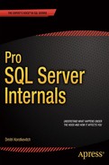
Every query submitted to SQL Server goes through a process of compilation and execution. That process consists of the steps shown in Figure 25-1.
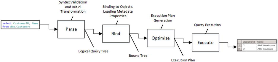
Figure 25-1. Query Life Cycle
When SQL Server receives a query, it goes through the parsing stage. SQL Server compiles and validates the query’s syntax and transforms it into a structure called a logical query tree. That tree consists of various logical relational algebraic operators, such as inner and outer joins, aggregations, and others.
In the next step, called binding, SQL Server binds logical tree nodes to the actual database objects, converting the logical tree to a bound tree. It validates that all objects referenced in the query are valid; that they exist in the database, and that all columns are correct. Finally, SQL Server loads various metadata properties associated with tables and columns, for example CHECK and NOT NULL constraints.
Query Optimizer uses the bound tree as input during the optimization stage, when the actual execution plan is generated. The execution plan is also a tree-like structure, which is comprised of physical operators and is used by SQL Server to execute a query. Physical operators perform the actual work during query execution, and they are different from logical operators. For example, a logical inner join can be transformed to one of three physical joins, including a nested loop, merge, or hash join.
One of the key elements that you need to remember is that Query Optimizer is not looking for the best execution plan that exists for the query. Query optimization is a complex and expensive process, and it is often impossible to evaluate all possible execution strategies.
For example, inner joins are commutative, and thus the result of (A join B) is equal to result of (B join A). Therefore, there are two possible ways that SQL Server can perform a two-table join; six ways that it can do three-table joins and N!, which is (N * (N - 1) * (N - 2) * ..) combinations for an N-table join. For a ten-table join, the number of possible combinations is 3,628,800, which is impossible to evaluate in a reasonable time period. Moreover, there are multiple physical join operators, which increase that number even further.
Optimization time is another important factor. For example, it is impractical to spend an extra ten seconds on optimization only to find an execution plan that saves just a fraction of a second during execution.
![]() Important The goal of Query Optimization is to find a good enough execution plan, quickly enough.
Important The goal of Query Optimization is to find a good enough execution plan, quickly enough.
SQL is declarative language in which you should focus on what needs to be done rather than how to achieve it. As a general rule, you should not expect that the way you wrote a query should affect the execution plan. SQL Server applies various heuristics that transform the query internally, removing contradicting parts, and changing join orders and performing other refactoring steps.
As with other general rules, they are correct only up to a degree. It is often possible to improve the performance of a query by refactoring and simplifying it, removing correlated subqueries, or splitting a complex query down into a few simple ones. As you know, cardinality estimation errors quickly progress and grow through the execution plan, which can lead to suboptimal performance, especially with very complex queries.
Moreover, you should not expect an execution plan for a particular query always to be the same and to rely on it as such. Query Optimizer algorithms change with every version of SQL Server and even with service pack releases. Even when this is not the case, statistics and data distribution changes lead to recompilation and potentially different execution plans.
![]() Note In some cases, you can use query and table hints and/or plan guides to control the execution plan shape. We will discuss table hints in more detail later in this chapter and plan guides in the following chapter.
Note In some cases, you can use query and table hints and/or plan guides to control the execution plan shape. We will discuss table hints in more detail later in this chapter and plan guides in the following chapter.
In the end, having the right indexes and efficient database schema is the best way to achieve predictability and good system performance. They simplify execution plans and make queries more efficient.
The query optimization process consists of the multiple phases, as shown in Figure 25-2.
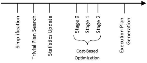
Figure 25-2. Query optimization phases
During the simplification stage, SQL Server transforms the query tree in a way that simplifies the optimization process further. Query Optimizer removes contradictions in the queries, performs computed column-matching, and works with joins, picking an initial join order based on the statistics and cardinality data.
Listing 25-1 provides an example of removing contradicting parts in a query. Both tables, NegativeNumbers and PositiveNumbers, have CHECK constraints that dictate the domain scope for the values. SQL Server can detect domain values contradictions, and it understands that an inner join operation will not return any data. It generates the execution plan, which does not access tables at all, as shown in Figure 25-3.
Listing 25-1. Removing contradicting parts from the execution plan
create table dbo.PositiveNumbers
(
        PositiveNumber int not null,

        constraint CHK_PositiveNumbers
        check (PositiveNumber > 0)
);

create table dbo.NegativeNumbers
(
        NegativeNumber int not null,

        constraint CHK_NegativeNumbers
        check (NegativeNumber < 0)
);

select *
from dbo.PositiveNumbers e join dbo.NegativeNumbers o on
        e.PositiveNumber = o.NegativeNumber
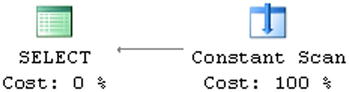
Figure 25-3. Execution plan for the query
After the simplification phase is completed, Query Optimizer checks if there is a trivial plan available for the query. This happens when a query has either only one plan available to execute, or when the choice of plan is obvious. Listing 25-2 shows such an example.
Listing 25-2. Query with trivial execution plan
create table dbo.Data
(
        ID int not null,
        Col1 int not null,
        Col2 int not null,
        constraint PK_Data
        primary key clustered(ID)
);

select * from dbo.Data where ID = 11111;
SQL Server generates the trivial execution plan, which uses a Clustered Index Seek operator, as shown in Figure 25-4.
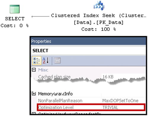
Figure 25-4. Trivial execution plan
Even though there are technically two different execution plan choices, Clustered Index Seek and Clustered Index Scan, Query Optimizer does not consider a scan option, because it is clearly more expensive. Moreover, adding a nonclustered index on Col1 or Col2 would introduce an additional, non-optimal execution plan choice. Nevertheless, Query Optimizer is still able to detect it and generate a trivial execution plan instead.
![]() Note You can check if an execution plan is trivial in the properties of the root operator or in XML representation of the plan.
Note You can check if an execution plan is trivial in the properties of the root operator or in XML representation of the plan.
If a trivial plan was not found, SQL Server checks if any auto-updated statistics are outdated and triggers a statistics update if needed. If the statistics need to be updated synchronously, which is the default option, Query Optimizer waits until the statitistics update is finished. Otherwise, an optimization is done based on old, outdated statistics, while statistics are updated asynchronously in another thread. After that, SQL Server starts a cost-based optimization, which includes a few different stages. Each stage explores more rules and as a consequence, it can take a longer time to execute.
- Stage 0 is called Transaction Processing, and it is targeted at scenarios that represent an OLTP workload with multiple (at least three) table joins, selecting a relatively small number of rows using indexes. This stage usually uses nested loop joins; although in some cases it may consider a hash join instead. Only a limited number of optimization rules are explored during this stage.
- Stage 1 is called Quick Plan, and it applies most of the optimization rules available in SQL Server. It may be run twice, looking for serial and parallel execution plans if needed. Most queries in SQL Server find the execution plan during this stage.
- Stage 2 is called Full Optimization, and it performs the most comprehensive and, therefore, longest running analysis, exploring all of the optimization rules available.
Each stage has its own entry and termination conditions. For example, Stage 0 requires a query to have at least three-table joins; otherwise, it will not be executed. Alternatively, if the cost of the plan exceeded some threshold during optimization, the stage is terminated and Query Optimizer moves on to the next, more comprehensive, stage. Optimization can be completed at any stage, as soon as a “good enough” plan is found.
You can examine the details of the optimization process by using undocumented trace flag 8675. The usual disclaimer about undocumented trace flags applies here: be careful, and do not use them in production. You also need to use trace flag 3604 to redirect output to the console.
Figure 25-5 illustrates the optimization statistics for one of the queries. As you can see, SQL Server performed Stage 0 and Stage 1 optimizations, generating the execution plan after Stage 1.
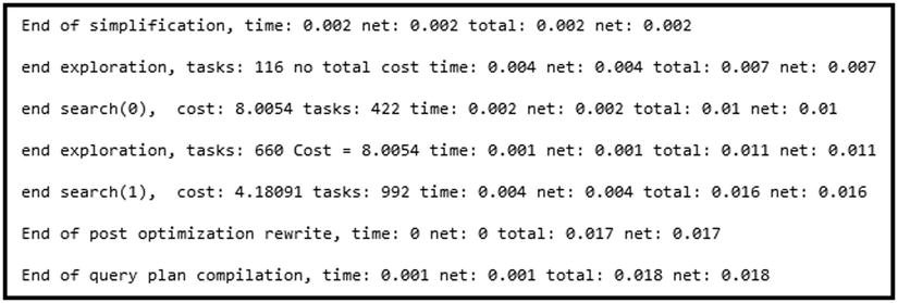
Figure 25-5. Optimization statistics returned by trace flag 8675
![]() Note The documented data management view sys.dm_exec_query_optimizer_info, allows you to retrieve Query Optimizer related statistics. While this DMV provides a great overview in server scope, it does not allow you to filter information for the specific session, which makes it very hard to use in busy environments. You can get more information about this DMV at: http://technet.microsoft.com/en-us/library/ms175002.aspx.
Note The documented data management view sys.dm_exec_query_optimizer_info, allows you to retrieve Query Optimizer related statistics. While this DMV provides a great overview in server scope, it does not allow you to filter information for the specific session, which makes it very hard to use in busy environments. You can get more information about this DMV at: http://technet.microsoft.com/en-us/library/ms175002.aspx.
Finally, when Query Optimizer is satisfied with the optimization results, it generates the execution plan.
As you can guess, SQL Server analyzes and explores a large number of alternative execution strategies during the query optimization stage. Those alternatives, which are part of the query tree, are stored in the part of Query Optimizer called Memo. SQL Server performs cost estimation for every group in Memo, which allows it to locate the least expensive alternative when generating an execution plan.
The cost calculation is based on a complex mathematical model, and it considers various factors, such as cardinality, row size, expected memory usage and number of sequential and random I/O operations, parallelism overhead, and others. The costing numbers and plan cost are meaningless by themselves; they should be used for comparison only.
There are quite a few assumptions in the costing model that help to make it more consistent.
- Random I/O is anticipated to be evenly distributed across the database files. For example, if an execution plan requires performing ten RID Lookup operations in a heap table, the costing model would expect that ten random physical I/O operations would be required. In reality, the data can reside on the same data pages, which can lead to a situation where Query Optimizer overcosts some operators in the plan.
- Query Optimizer expects all queries to start with cold cache and perform physical I/O when accessing the data. This may be incorrect in production systems when data pages are often cached in the buffer pool. In some rare cases, it could lead to a situation where SQL Server chooses a less efficient plan that requires less I/O at the cost of higher CPU or memory usage.
- Query Optimizer assumes that sequential I/O performance is significantly faster than random I/O performance. While this is usually true for magnetic hard drives, it is not exactly the case with solid-state media, where random I/O performance is much closer to sequential I/O, as compared to magnetic hard drives. SQL Server does not take drive type into account, and overcosts random I/O operations in the case of solid-state based disk arrays. It can generate execution plans with a Clustered Index Scan instead of Nonclustered Index Seek and Key Lookup, which could be less efficient with SSD-based disk subsystems for some of the queries. It is also worth noting that the same could happen with modern high-performance disk arrays with a large number of drives and very good random I/O performance.
With all that being said, the costing model in SQL Server generally produces correct and consistent results. However, as with any mathematical model, the quality of the output highly depends on the quality of the input data. For example, it is impossible to provide correct cost estimations when the cardinality estimations are incorrect due to outdated statistics. Keeping statistics up to date helps SQL Server generate efficient execution plans.
SQL Server generates an execution plan in the final stage of query optimization. The execution plan is passed to the Query Executor, which, as you can guess by its name, executes the query.
The execution plan is a tree-like structure that includes a set of operators, sometimes called iterators. Typically, SQL Server uses a row-based execution model, where each operator generates a single row by requesting the rows from one or more children and passes the generated row to its parent.
![]() Note SQL Server 2012 introduced a new “batch-mode” execution model, which is used with some Data Warehouse queries. We will talk about this execution model in Chapter 34, “Introduction to ColumnStore Indexes.”
Note SQL Server 2012 introduced a new “batch-mode” execution model, which is used with some Data Warehouse queries. We will talk about this execution model in Chapter 34, “Introduction to ColumnStore Indexes.”
Let’s look at an example that illustrates a row-based execution model, assuming that you have the query shown in Listing 25-3.
Listing 25-3. Row-based execution: Sample query
select top 10 c.CustomerId, c.Name, a.Street, a.City, a.State, a.ZipCode
from
        dbo.Customers c join dbo.Addresses a on
                c.PrimaryAddressId = a.AddressId
order by
        c.Name
This query would produce the execution plan shown in Figure 25-6. SQL Server selects all of the data from the Customers table, sorts it based on the Name column, getting the first 10 rows, joins it with the Addresses data, and returns it to the client.
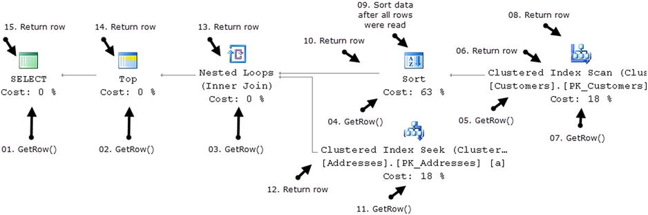
Figure 25-6. Row-based model: Getting the first row in the output
Let’s look how SQL Server executes such a query on operator-by-operator basis. The Select operator, which is the parent operator in the execution plan, calls the GetRow() method of the Top operator. The Top operator, in turn, calls the GetRow() method of the Nested Loop Join.
As you know, a Join needs to get data from two different sources to produce output. As a first step, it calls the GetRow() method of the Sort operator. In order to do sorting, SQL Server needs to read all of the rows first, therefore the Sort operation calls the GetRow() method of the Clustered Index Scan operator multiple times, accumulating the results. The Scan operator, which is the lowest operator in the execution plan tree, returns one row from the Customers table per call. Figure 25-6 shows just two GetRow() calls for simplicity’s sake.
When all of the data from the Customers table has been read, the Sort operator performs sorting and returns the first row back to the Join operator, which calls the GetRow() method of the Clustered Index Seek operator on the Addresses table after that. If there is a match, the Join operator concatenates data from both inputs and passes the resulting row back to the Top operator, which, in turn, passes it to Select.
The Select operator returns a row to the client and requests the next row by calling the GetRow() method of the Top operator again. The process repeats until the first 10 rows are selected. It is worth mentioning that the operators kept their state and the Sort operator preserves the sorted data and can return all subsequent rows without accessing the Clustered Index Scan operator, as shown in Figure 25-7.
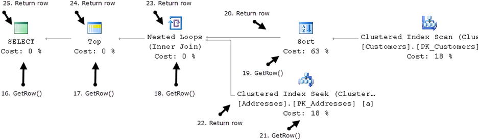
Figure 25-7. Row-based model: Getting the subsequent row
![]() Note There are two other methods Open() and Close() called for each operator during execution. The Open() method initializes the operator before first the GetRow() call. The Close() method performs clean up at the end of the execution.
Note There are two other methods Open() and Close() called for each operator during execution. The Open() method initializes the operator before first the GetRow() call. The Close() method performs clean up at the end of the execution.
As you probably noticed, there are two kinds of operators. The first group, called non-blocking operators, consumes the row from the children and produces the output immediately. The second group, called blocking operators, must consume all rows from the children before producing the output. In our example, the Sort operator is the only blocking operator, which consumes all Customers table rows before sorting it.
Even though blocking operators are completely normal and cannot be avoided in many cases, there are a couple of issues associated with them. The first issue is memory usage. Every operator, blocking or non-blocking, requires some memory to execute; however, blocking operators can use a large amount of memory when they accumulate and process rows.
Each query requests a memory grant from SQL Server for the execution. The amount of memory required for the operators is the most important factor that affects its size. Internally, SQL Server arranges queries among three different pools based on the amount of memory that they request. Queries in the highest memory-consuming pool generally wait longer for the memory to be granted.
![]() Tip You can monitor memory grant requests with the sys.dm_exec_query_memory_grants DMV. You can also monitor various performance counters in the Memory Manager object in the System Performance Monitor.
Tip You can monitor memory grant requests with the sys.dm_exec_query_memory_grants DMV. You can also monitor various performance counters in the Memory Manager object in the System Performance Monitor.
Correct memory size estimation is very important. Overestimation and underestimation both negatively affect the system. Overestimation wastes server memory, and it can increase how long a query waits for memory grant. Underestimation, on the other hand, can force SQL Server to perform sorting or hashing operations in tempdb rather than in-memory, which is significantly slower.
Memory estimation for an operator depends on the cardinality and average row size estimation. Either error leads to an incorrect memory grant request. The typical sources of cardinality estimation errors are inaccurate statistics and/or Query Optimizer model limitations. They can often be addressed by statistics maintenance and query simplification and optimization. However, dealing with row size estimation errors is a bit trickier.
SQL Server knows the size of the fixed-length data portion of the row. For variable-length columns, however, it estimates that data is populated on average 50 percent of the defined column size. For example, if you had two columns defined as varchar(100) and nvarchar(200), SQL Server would estimate that every data row stores 50 and 200 bytes in those columns respectively. For (n)varchar(max) and varbinary(max) columns, SQL Server uses 4,000 bytes as the base figure.
![]() Tip You can improve row size estimation by defining variable-length columns two times larger than the average size of the data stored there.
Tip You can improve row size estimation by defining variable-length columns two times larger than the average size of the data stored there.
Let’s look at an example and create two tables, as shown in Listing 25-4.
Listing 25-4. Variable-length columns and memory grant: Table creation
create table dbo.Data1
(
        ID int not null,
        Value varchar(100) not null,
        constraint PK_Data1
        primary key clustered(ID)
);

create table dbo.Data2
(
        ID int not null,
        Value varchar(200) not null,
        constraint PK_Data2
        primary key clustered(ID)
);

;with N1(C) as (select 0 union all select 0) -- 2 rows
,N2(C) as (select 0 from N1 as T1 cross join N1 as T2) -- 4 rows
,N3(C) as (select 0 from N2 as T1 cross join N2 as T2) -- 16 rows
,N4(C) as (select 0 from N3 as T1 cross join N3 as T2) -- 256 rows
,N5(C) as (select 0 from N4 as T1 cross join N4 as T2 ) -- 65,536 rows
,Nums(Num) as (select row_number() over (order by (select null)) from N5)
        insert into dbo.Data1(ID, Value)
                select Num , replicate('0',100)
                from Nums;

insert into dbo.Data2(ID, Value)
        select ID, Value from dbo.Data1;
In the next step, let’s run two identical queries against those tables, as shown in Listing 25-5. I am using the variable as a way to discard the result set.
Listing 25-5. Variable-length columns and memory grant: Queries
declare
        @V varchar(200)

select @V = Value
from dbo.Data1
where ID < 42000
order by Value, ID desc

select @V = Value
from dbo.Data2
where ID < 42000
order by Value, ID desc
As you can see in Figure 25-8, an incorrect memory grant forced SQL Server to spill data to tempdb, which increases the execution time.
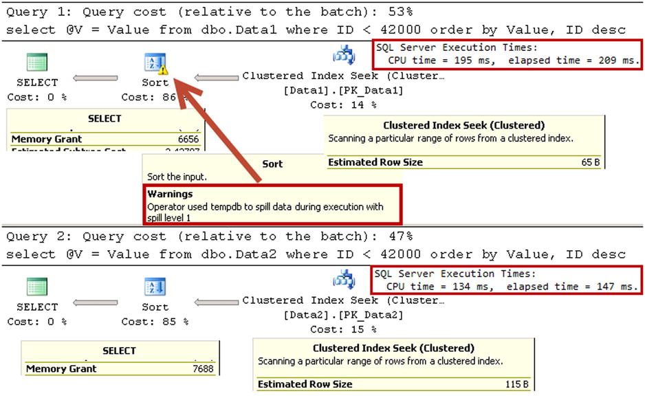
Figure 25-8. Variable-length columns and memory grant: Execution Plan
![]() Tip You can monitor data spills to tempdb with Sort and Hash Warnings in SQL Trace and Extended Events.
Tip You can monitor data spills to tempdb with Sort and Hash Warnings in SQL Trace and Extended Events.
Blocking operators can negatively affect the performance of queries when they are present in parallel sections of the execution plan. The parallelism operator, which merges data from parallel executing threads, would wait until all threads finish their execution. Thus the execution time would depend on the slowest thread. Blocking operators can contribute to delays especially in the case of tempdb spills. Such conditions often happen when a parallel thread workload has been unevenly distributed due to cardinality estimation errors.
![]() Tip You can see the distribution of workload between threads when you open the “Properties” window for the operators in the parallel section of the graphical execution plan in SQL Server Management Studio.
Tip You can see the distribution of workload between threads when you open the “Properties” window for the operators in the parallel section of the graphical execution plan in SQL Server Management Studio.
In some cases, adding indexes can remove blocking operators from execution plans. For example, if you added the index CREATE INDEX IDX_Customers_Name ON dbo.Customers(Name), SQL Server would not need to sort customer’ data anymore and the query from Listing 25-3 would end up with an execution plan without blocking operators, as shown in Figure 25-9.
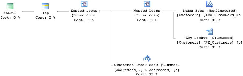
Figure 25-9. Execution plan without blocking operators
There are three ways that you can analyze execution plans in SQL Server and Management Studio. The most common method is graphical execution plan representation, which can be enabled through the “Include Actual Execution Plan” menu item in the Query menu. A graphical execution plan represents an execution plan tree rotated 90 degrees counter-clockwise. The top root element of the tree is the leftmost icon on the plan, with children nodes on the right side of the parents.
When you select an operator in the plan, a small pop-up window shows some of the properties of the operator. However, you can get a more comprehensive picture by opening the operator’s Properties window in Management Studio.
![]() Tip SQL Sentry “Plan Explorer” is a great freeware tool, which simplifies execution plan analysis and addresses a few of the shortcomings of SQL Server Management Studio. You can download it from http://sqlsentry.net.
Tip SQL Sentry “Plan Explorer” is a great freeware tool, which simplifies execution plan analysis and addresses a few of the shortcomings of SQL Server Management Studio. You can download it from http://sqlsentry.net.
In addition to a graphical representation of the execution plan, SQL Server can display it as text or as XML. A text representation places each operator into individual lines displaying parent/child relationships with indents and | symbols. A text execution plan may be useful when you need to share a compact and easy-to-understand representation of the execution plan without worrying about image size and the scale of the graphical execution plan.
An XML execution plan represents operators as XML nodes with child operator nodes nested in parent nodes. It is the most complete representation of the execution plan, which includes a large set of attributes, which are omitted in other modes. However, an XML execution plan is complex and it requires some time and practice before it can become easy to understand.
In addition to the actual execution plan, SQL Server can provide an estimated execution plan without running the actual query. This allows you to obtain the execution plan shape quickly for analysis. However, it does not include actual row and execution counts, which are very helpful during query performance tuning.
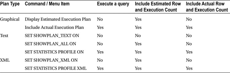
Table 25-1 shows different commands that generate estimated and actual execution plans in graphical, text, and XML modes.
Table 25-1. Commands that generate actual and estimated execution plans
![]() Important One of the key metrics to which you should pay attention when analyzing execution plans is the difference between actual and estimated row counts. A large discrepancy between these two values is often a sign of cardinality estimation errors due to inaccurate statistics.
Important One of the key metrics to which you should pay attention when analyzing execution plans is the difference between actual and estimated row counts. A large discrepancy between these two values is often a sign of cardinality estimation errors due to inaccurate statistics.
SQL Server uses two types of operators: logical and physical. These operators are used during the different stages of the Query Life Cycle in different types of query trees. SQL Server uses logical operators during the parsing and binding stages and replaces them with physical operators during optimization. For example, an inner join logical operator can be replaced with one of three physical join operators in the execution plan.
It is impossible to cover all physical operators in this chapter, however we will discuss a few common ones that you will often encounter in execution plans.
There are multiple variations of physical join operators in SQL Server, which dictate how join predicates are matched and what is included in the resulting row. However, in terms of algorithms, there are just three join types: nested loop, merge, and hash joins.
A nested loop join is simplest join algorithm. As with any join type, it accepts two inputs, which are called outer and inner tables. The algorithm for an inner nested loop join is shown in Listing 25-6, and the algorithm for an outer nested loop join is shown in Listing 25-7.
Listing 25-6. Inner nested loop join algorithm
for each row R1 in outer table
        for each row R2 in inner table
                if R1 joins with R2
                        return join (R1, R2)
Listing 25-7. Outer nested loop join algorithm
for each row R1 in outer table
        for each row R2 in inner table
                if R1 joins with R2
                        return join (R1, R2)
                else
                        return join (R1, NULL)
As you can see, the cost of the algorithm depends on the size of the inputs, and it is proportional to its multiplication; that is, the size of the outer input multiplied by the size of the inner input. The cost grows quickly with the size of the inputs; therefore, a nested loop join is efficient when at least one of the inputs is small.
A nested loop join does not require join keys to have an equality predicate. SQL Server evaluates a join predicate between every row from both inputs. In fact, it does not require a join predicate at all. For example, the CROSS JOIN logical operator would lead to a nested loop physical join when every row from both inputs are joined together.
The merge join works with two sorted inputs. It compares two rows, one at time, and returns their join to the client if they are equal. Otherwise, it discards the lesser value and moves on to the next row in the input.
Contrary to nested loop joins, a merge join requires at least one equality predicate on the join keys. Listing 25-8 shows the algorithm for the inner merge join.
Listing 25-8. Inner merge join algorithm
/* Prerequirements: Inputs I1 and I2 are sorted */
get first row R1 from input I1
get first row R2 from input I2
while not end of either input
begin
        if R1 joins with R2
        begin
                return join (R1, R2)
                get next row R2 from I2
        end
        else if R1 < R2
                get next row R1 from I1
        else /* R1 > R2 */
                get next row R2 from I2
end
The cost of the merge join algorithm is proportional to the sum of the sizes of both inputs, which makes it more efficient on large inputs as compared to a nested loop join. However, a merge join requires both inputs to be sorted, which is often the case when inputs are indexed on the join key column.
In some cases, however, SQL Server may decide to sort input(s) using the Sort operator before a merge join. The cost of the sort obviously needs to be factored together with the cost of the join operator during its analysis.
![]() Tip In some cases, you can eliminate the Sort operator by creating corresponding indexes that pre-sort the data.
Tip In some cases, you can eliminate the Sort operator by creating corresponding indexes that pre-sort the data.
Unlike the nested loop join, which works best on small inputs, and merge join, which excels on sorted inputs, a hash join is designed to handle large unsorted inputs. The hash join algorithm consists of two different phases.
During the first, or build, phase, a hash join scans one of inputs, calculates the hash values of the join key, and places it into the hash table. Next, in the second, or probe, phase, it scans the second input, and checks, or probes, if the hash value of the join key from second input exists in the hash table. When this is the case, SQL Server evaluates the join predicate for the row from the second input and all rows from the first input, which belong to the same hash bucket.
This comparison must be done because the algorithm that calculates the hash values does not guarantee the uniqueness of the hash value of individual keys, which leads to hash collision when multiple different keys generate the same hash. Even though there is the possibility of additional overhead from the extra comparison operations due to hash collisions, those situations are relatively rare.
Listing 25-9 shows the algorithm of an inner hash join.
Listing 25-9. Inner hash join algorithm
/* Build Phase */
for each row R1 in input I1
begin
        calculate hash value on R1 join key
        insert hash value to appropriate bucket in hash table
end
/* Probe Phase */
for each row R2 in input I2
begin
        calculate hash value on R2 join key
        for each row R1 in hash table bucket
                if R1 joins with R2
                        return join (R1, R2)
end
As you can guess, a hash join requires memory to store the hash table. The performance of a hash join greatly depends on correct memory grant estimation. When the memory estimation is incorrect, the hash join stores some hash table buckets in tempdb, which can greatly reduce the performance of the operator.
When this happens, SQL Server tracks where the buckets are located: either in-memory or on-disk. For each row from the second input, it checks where the hash bucket is located. If it is in-memory, SQL Server processes the row immediately. Otherwise, it stores the row in another internal temporary table in tempdb.
After the first pass is done, SQL Server discards in-memory buckets, replacing them with the buckets from disk and repeats the probe phase for all of the remaining rows from the second input that were stored in the internal temporary table. If there still weren’t enough memory to accommodate all hash buckets, some of them would be spilled on-disk again.
The number of times when this happens is called the recursion level. SQL Server tracks it and, eventually, switches to a special bailout algorithm, which is less efficient, although it’s guaranteed to complete at some point.
![]() Tip You can monitor hash table spills to tempdb with Hash Warnings in SQL Trace and Extended Events.
Tip You can monitor hash table spills to tempdb with Hash Warnings in SQL Trace and Extended Events.
Similar to a merge join, hash joins require at least one equality predicate in the join condition.
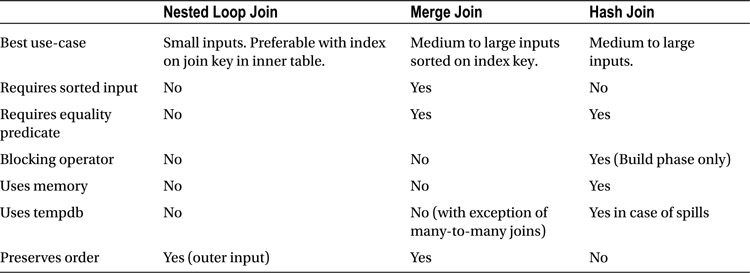
As usual, the choice of the join operator fits into the “It Depends” category. Each join type has its own pros and cons, which makes it good for some use-cases and not so good for others.
Table 25-2 compares different join types in various scenarios.
Table 25-2. Join types comparison
One of the common mistakes people make during performance tuning is relying strictly on the number of logical reads produced by the query. Even though that number is a great performance characteristic, it could be misleading in the case of joins. For example, it is entirely possible that a hash join produces fewer reads as compared to a nested loop. However, it would not factor in CPU usage and memory overhead or the performance implication in the case of tempdb spills and bailouts.
The merge join is another great example. While it is more efficient than a nested loop on sorted inputs, it is easy to overlook the overhead of the Sort operation, which often prepares input for the merge join.
As usual, you should keep join behaviors and the pros and cons of each join type in mind, and factor this into your analysis.
Aggregates perform a calculation on the set of values and return a single value. A typical example of aggregates in SQL is the MIN() function, which returns the minimal value from the group of values it processes.
SQL Server supports two types of aggregate operators: stream and hash aggregates.
A stream aggregate performs the aggregation based on sorted input, for example, when data is sorted on a column, which is specified in a group by clause. Listing 25-10 shows the stream aggregate algorithm.
Listing 25-10. Stream Aggregate algorithm
/* Prerequirement: input is sorted */
for each row R1 from input
begin
        if R1 does not match current group by criteria
        begin
                return current aggregate results (if any)
                clear current aggregate results
                set current group criteria to match R1
        end
        update aggregate results with R1 data
end
return current aggregate results (if any)
Due to the sorted input requirement, SQL Server often uses a stream aggregate together with the Sort operator. Let’s look at an example and create a table with some sales information for a company. After that, let’s run the query, which calculates total amount of sales for each customer. The code to perform this is shown in Listing 25-11.
Listing 25-11. Query that uses stream aggregate
create table dbo.Orders
(
        OrderID int not null,
        CustomerId int not null,
        Total money not null,
        constraint PK_Orders
        primary key clustered(OrderID)
);

;with N1(C) as (select 0 union all select 0) -- 2 rows
,N2(C) as (select 0 from N1 as T1 cross join N1 as T2) -- 4 rows
,N3(C) as (select 0 from N2 as T1 cross join N2 as T2) -- 16 rows
,N4(C) as (select 0 from N3 as T1 cross join N3 as T2) -- 256 rows
,Nums(Num) as (select row_number() over (order by (select null)) from N4)
        insert into dbo.Orders(OrderId, CustomerId, Total)
                select Num, Num % 10 + 1, Num
                from Nums;

select Customerid, sum(Total) as [Total Sales]
from dbo.Orders
group by CustomerId
You can see the execution plan of the query in Figure 25-10. There is no index on the CustomerId column, and SQL Server needs to add a Sort operator to guarantee sorted input for the Stream Aggregate operator.
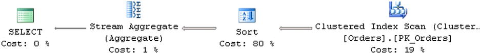
Figure 25-10. Execution plan of the query with Stream Aggregate
A hash aggregate is very similar to a hash join. It is targeted towards large input and requires memory to store the hash table. The hash aggregate algorithm is shown in Listing 25-12.
Listing 25-12. Hash Aggregate algorithm
for each row R1 from input
begin
        calculate hash value of R1 group columns
        check for a matching row in hash table
        if matching row exists
                update aggregate results of matching row
        else
                insert new row into hash table
end
return all rows from hash table with aggregate results
Similar to a hash join, a hash table can be spilled to tempdb, which negatively affects the performance of the aggregate.
Comparing Aggregates
As with joins, stream and hash aggregates are targeted towards different use-cases. A stream aggregate works best with sorted input—either because of existing indexes or when the amount of data is small and can be easily sorted. A hash aggregate, on the other hand, is targeted towards large unsorted inputs.
Table 25-3 compares hash and stream aggregates.
Table 25-3. Aggregate comparison
Stream Aggregate |
Hash Aggregate |
|
|---|---|---|
Best use-case |
Small size input where data can be sorted with the Sort operator or pre-sorted input. |
Medium-to-large unsorted input. |
Requires sorted input |
Yes |
No |
Blocking |
No. However it often requires a blocking Sort operator. |
Yes |
Uses memory |
No |
Yes |
Uses tempdb |
No |
Yes in case of spills |
You should consider the cost of the Sort operator during performance tuning if it is used only to support a stream aggregate pre-requirement. The cost of sorting usually exceeds the cost of stream aggregation itself. You can often remove it by creating indexes, which would sort the data in the order required for a stream aggregate.
Spools
Spool operators, in a nutshell, are internal in-memory or on-disk caches/temporary tables. SQL Server often uses spools for performance reasons to cache the results of complex subexpressions that need to be used several times during query execution.
Let’s look at an example and use the table we created in Listing 25-11. We will run the query that returns information about all of the orders, together with the total amount of sales on a per-customer basis, as shown in Listing 25-13.
Listing 25-13. Table Spool example
select OrderId, CustomerID, Total
        ,Sum(Total) over(partition by CustomerID) as [Total Customer Sales]
from dbo.Orders
The execution plan for the query is shown in Figure 25-11. As you can see, SQL Server scans the table, sorts the data based on the CustomerID order, and uses a Table Spool operator to cache the results. This allows SQL Server to access the cached data and avoid an expensive sorting operation later.
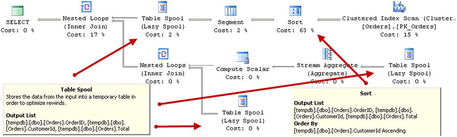
Figure 25-11. Execution plan of the query
Even though a Table Spool operator is shown in the execution plan several times, it is essentially the same spool/cache. SQL Server builds it the first time and uses its data later.
As a side note, this is a great example of the declarative nature of SQL. The query in Listing 25-14 is the logical equivalent of the query in Listing 25-13, and both of them have the same execution plan.
Listing 25-14. Alternative version of the query
select o.OrderId, o.CustomerID, o.Total, ot.Total
        ,os.TotalSales as [Total Customer Sales]
from
        dbo.Orders o join
        (
                select customerid, sum(total) as TotalSales
                from dbo.Orders
                group by CustomerID
        ) ot on
                o.CustomerID = ot.CustomerID
SQL Server uses spools for Halloween Protection when modifying the data. Halloween Protection helps you avoid situations where data modifications affect what data need to be updated. The classic example of such a situation is shown in Listing 25-15. Without Halloween Protection, the insert statement would fall into an infinite loop, reading the rows it has been inserting.
Listing 25-15. Halloween Protection
create table dbo.HalloweenProtection
(
        Id int not null identity(1,1),
        Data int not null
);

insert into dbo.HalloweenProtection(Data)
        select Data from dbo.HalloweenProtection;
The execution plan of the insert statement is shown in Figure 25-12. SQL Server uses the Table Spool operator to cache the data from the table prior to insert beginning to avoid an infinite loop during execution.

Figure 25-12. Halloween Protection execution plan
As I mentioned in Chapter 10, “User-Defined Functions,” it is important to use the WITH SCHEMABINDING option when you define scalar user-defined functions. This option forces SQL Server to analyze if a user-defined function performs data access and avoids extra Halloween Protection-related Spool operators in the execution plan.
Listing 25-16 shows an example of the code that creates two user-defined functions, using them in where clause of update statements.
Listing 25-16. Halloween Protection and user-defined functions
create function dbo.ShouldUpdateData(@Id int)
returns bit
as
begin
        return (1)
end
go

create function dbo.ShouldUpdateDataSchemaBound(@Id int)
returns bit
with schemabinding
as
begin
        return (1)
end
go

update dbo.HalloweenProtection
set Data = 0
where dbo.ShouldUpdateData(ID) = 1;

update dbo.HalloweenProtection
set Data = 0
where dbo.ShouldUpdateDataSchemaBound(ID) = 1;
Neither of these functions accesses the data, and therefore cannot introduce the Halloween effect. However, SQL Server does not know that in the case of non-schema bound functions, and it adds a Spool operator to execution plan, as shown in Figure 25-13.
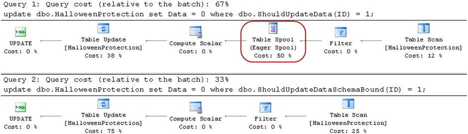
Figure 25-13. Halloween Protection and user-defined functions: Execution plans
Spool temporary tables are usually referenced as worktables in the I/O statistics for the queries. You should analyze table spool-related reads during query performance tuning. While spools can improve the performance of queries, there is overhead introduced by the unnecessary spools. You can often remove them by creating appropriate indexes on the tables.
SQL Server can execute queries using multiple CPUs simultaneously. Even though parallel query execution can reduce the response time of queries, it comes at a cost. Parallelism always introduces the overhead of managing multiple threads.
Let’s look at an example and create two tables, as shown in Listing 25-17. The script inserts 65,536 rows into table dbo.T1 and 1,048,576 rows into table dbo.T2.
Listing 25-17. Parallelism: Table creation
create table dbo.T1
(
        T1ID int not null,
        PlaceHolder char(100),
        constraint PK_T1
        primary key clustered(T1ID)
);

create table dbo.T2
(
        T1ID int not null,
        T2ID int not null,
        PlaceHolder char(100)
);

create unique clustered index IDX_T2_T1ID_T2ID
on dbo.T2(T1ID, T2ID);

;with N1(C) as (select 0 union all select 0) -- 2 rows
,N2(C) as (select 0 from N1 as T1 cross join N1 as T2) -- 4 rows
,N3(C) as (select 0 from N2 as T1 cross join N2 as T2) -- 16 rows
,N4(C) as (select 0 from N3 as T1 cross join N3 as T2) -- 256 rows
,N5(C) as (select 0 from N4 as T1 cross join N4 as T2) -- 65,536 rows
,Nums(Num) as (select row_number() over (order by (select null)) from N5)
        insert into dbo.T1(T1ID)
                select Num from Nums;

;with N1(C) as (select 0 union all select 0) -- 2 rows
,N2(C) as (select 0 from N1 as T1 cross join N1 as T2) -- 4 rows
,N3(C) as (select 0 from N2 as T1 cross join N2 as T2) -- 16 rows
,Nums(Num) as (select row_number() over (order by (select null)) from N3)
        insert into dbo.T2(T1ID, T2ID)
                select T1ID, Num
                from dbo.T1 cross join Nums;
In the next step, let’s run two selects, as shown in Listing 25-18.
Listing 25-18. Parallelism: Test queries
select count(*)
from
        (
                select t1.T1ID, count(*) as Cnt
                from dbo.T1 t1 join dbo.T2 t2 on
                        t1.T1ID = t2.T1ID
                group by t1.T1ID
        ) s
option (maxdop 1);

select count(*)
from
        (
                select t1.T1ID, count(*) as Cnt
                from dbo.T1 t1 join dbo.T2 t2 on
                        t1.T1ID = t2.T1ID
                group by t1.T1ID
        ) s
We would force a serial execution plan for the first query using MAXDOP 1 as a query hint. The second query would have a parallel execution plan. Figure 25-14 illustrates this scenario.
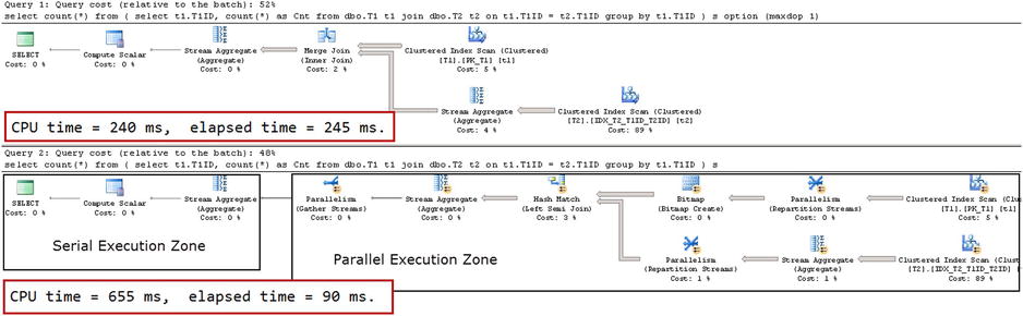
Figure 25-14. Parallel Execution: Query Plans
As you can see, the response (elapsed) time of the first query is much slower than that of the second query: 245 milliseconds versus 90 milliseconds. However, the total CPU time of the first query is much lower compared to second query: 240 milliseconds versus 655 milliseconds. We are using CPU resources for parallelism management.
A parallel execution plan does not necessarily mean that all operators are executing in parallel. An execution plan can have both parallel and serial execution zones. The parallel plan shown in Figure 25-14 runs a subquery in a parallel zone and an outer count(*) calculation serially.
The Parallelism operator, sometimes called Exchange, manages parallelism during query execution, and it can run in three different modes. It accepts the input data from one or more producer threads and distributes it across one or more consumer threads. Let’s take an in-depth look at those modes.
In Distribute Streams mode, the Parallelism operator accepts data from one producer thread and distributes it across multiple consumer threads. This mode is usually the entry point to the parallel execution zone in the plan. Figure 25-15 illustrates this concept.
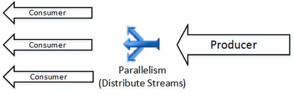
Figure 25-15. Parallelism: Distribute Streams
In Gather Streams mode, the Parallelism operator merges the data from multiple producer threads and passes it to a single consumer thread. This mode is usually the exit point from the parallel execution zone in the plan. Figure 25-16 illustrates this idea.
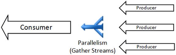
Figure 25-16. Parallelism: Gather Streams
Finally, in Repartition Streams mode, the Parallelism operator accepts data from multiple producer threads and distributes it across multiple consumer threads. This happens in the middle of a parallel zone of the plan when the data needs to be redistributed between execution threads. Figure 25-17 illustrates this concept.
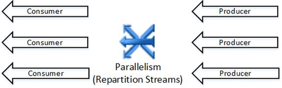
Figure 25-17. Parallelism: Repartition Streams
There are several different ways that data can be distributed between consumer threads. Table 25-4 summarizes these methods.
Table 25-4. Data redistribution methods in parallelism
Redistribution Method |
Description |
|---|---|
Broadcast |
Send row to all consumer threads |
Round Robin |
Send row to the next consumer thread in sequence |
Demand |
Send row to the next consumer thread that requests the row |
Range |
Use range function to determine which consumer thread should get a row |
Hash |
Use hash function to determine which consumer thread should get a row |
The Parallelism operator uses a different execution model than other operators. It uses a push-based model, with producer threads pushing rows to it. It is the opposite of a pull-based model, where the parent operator calls the GetRow() method of a child operator to get the data.
Evenly distributed workload is the key element for good performance of parallel execution plans. You can see the number of rows processed by each thread in the “Actual Number of Rows” section of the Properties window in Management Studio. That information is not displayed in a tool-tip in the graphical execution plans. Thread 0 is the parallelism management thread, which always shows zero as number of rows.
Uneven data distribution and outdated statistics are common causes of uneven workload distribution between threads. Figure 25-18 shows how workload distribution changes after a statistics update on one of the tables. The left side shows the distribution before the statistics update and the right side shows it after the update.
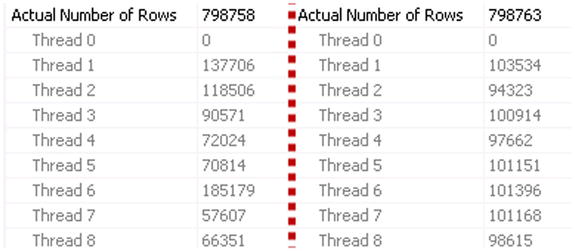
Figure 25-18. Workload distribution before and after a statistics update
![]() Note We will discuss best practices and other parallelism-related questions in Chapter 27, “System Troubleshooting.”
Note We will discuss best practices and other parallelism-related questions in Chapter 27, “System Troubleshooting.”
Query Optimizer usually does a good job of generating decent execution plans. However, in some cases, you can decide to fine-tune the shape of the execution plan with query and table hints. For example, query and table hints allow you to force Query Optimizer to choose specific indexes or join types for the query.
Query hints are a great, but very dangerous, tool. While on the one hand they can help you improve the quality of execution plans, they could significantly decrease the performance of the system when applied incorrectly on the other. You should have a very good understanding of how SQL Server works and know your system and data if you decide to use them.
The supportability of the system is another very important factor. You should document the cases when hints are used and periodically re-evaluate if they are still required. The amount of data and data distribution changes can lead to situations where plans forced by the hints become suboptimal. For example, consider the situation when a hint forces Query Optimizer to use a nested loop join. This join type will work inefficiently as the amount of data and size of inputs grows.
Forcing Query Optimizer to use a specific index is another example. The choice of index can become inefficient in the case of data selectivity changes, and it would prevent Query Optimizer from using other indexes, which were created later. Moreover, the code would be broken and queries would error out if you ever dropped or renamed the index referenced by the hint.
As a general rule, you should only use hints as a last resort. If you do, make sure that the statistics are up to date and that the query cannot be optimized, simplified, or refactored before applying them.
In the case of parameter sniffing, it is usually better to use the OPTIMIZE FOR hint or statement-level recompile rather than force specific index usage with an index hint. We will discuss these approaches in greater depth in the next chapter.
INDEX is, perhaps, one of the most commonly used Query Hints, which forces Query Optimizer to use a specific index for data access. It requires you to specify either the name or id of the index as a parameter. In most cases, the name of the index is the better choice for supportability reasons. There are two exceptions, however, where index id is the better option, forcing the use of a clustered index or heap table scan. You can consider using 1 and 0 respectively as an id in those cases.
SQL Server can use either Scan or Seek access methods with an index. Listing 25-19 shows an example of INDEX hint usage, which forces SQL Server to use the IDX_Orders_OrderDate index in the query.
Listing 25-19. INDEX Query Hint
select OrderId, OrderDate, CustomerID, Total
from dbo.Orders with (Index = IDX_Orders_OrderDate)
where OrderDate between @StartDate and @EndDate
One of the legitimate use-cases for an INDEX query hint is forcing SQL Server to use one of the composite indexes in those cases where correct cardinality estimation is impossible. Consider the case when a table stores location information for multiple devices that belong to different accounts, as shown in Listing 25-20. Let’s assume that DeviceId is unique only within a single account.
Listing 25-20. Composite indexes and uneven data distribution: Table Creation
create table dbo.Locations
(
        AccountId int not null,
        DeviceId int not null,
        UtcTimeTag datetime2(0) not null,
        /* Other Columns */
);

create unique clustered index IDX_Locations_AccountId_UtcTimeTag_DeviceId
on dbo.Locations(AccountId, UtcTimeTag, DeviceId);

create unique nonclustered index IDX_Locations_AccountId_DeviceId_UtcTimeTag
on dbo.Locations(AccountId, DeviceId, UtcTimeTag);
The table stores information for multiple accounts, and it is common to have data distributed very unevenly in such a scenario where some accounts have hundreds or even thousands of devices while others have just a few of them. Let’s assume that we would like to select the data that belongs to a subset of devices for a specific time frame, as shown in Listing 25-21.
Listing 25-21. Composite indexes and uneven data distribution: Query
select *
from dbo.Locations
where
        AccountId = @AccountID and
        UtcTimeTag between @StartTime and @StopTime and
        DeviceID in (select DeviceID from #ListOfDevices);
SQL Server has two different choices for the execution plan. The first choice uses Nonclustered Index Seek and Key Lookup, which is better when you need to select data for a very small percent of the devices from the account. In all other cases, it is more efficient to use Clustered Index Seek with AccountId and UtcTimeTag as seek predicates, and to perform a range scan for all devices that belong to the account.
Unfortunately, SQL Server would not have enough data to perform correct cardinality estimation in either case. It can estimate the selectivity of particular AccountID data based on the histogram from either index; however, it is not enough to estimate cardinality for the list of devices.
One possible solution is to write the code that calculates the number of devices in the #ListOfDevices table and compare it to the total number of devices per account, forcing SQL Server to use a specific index with an INDEX hint based on the comparison results.
It is worth mentioning that such a system design is not optimal. It would be better to make DeviceId unique system-wide rather than in the account scope. This would allow you to make DeviceId the leftmost column in the nonclustered index, which can help SQL Server with cardinality estimations based on the list of devices. This approach, however, would still not factor time parameters into such estimations.
A FORCE ORDER query hint preserves the join order in the query. When this hint is specified, SQL Server always joins tables in the order in which joins are listed in the from clause of the query. However, SQL Server would choose the least-expensive join type in each case.
Listing 25-22 shows an example of such a hint. SQL Server will perform joins in the following order: ((TableA join TableB) join TableC).
Listing 25-22. FORCE ORDER hint
select *
from
        TableA join TableB on TableA.ID = TableB.AID
        join TableC on TableB.ID = TableC.BID
option (force order)
LOOP, MERGE, and HASH JOIN Hints
You can specify join types with LOOP, MERGE, and HASH hints on both query and individual join levels. It is possible to specify more than one join type in the query hint and allow SQL Server to choose the least-expensive one. A join operator hint takes precedence over a query hint if both are specified. Finally, a join type hint also forces join orders similarly to a FORCE ORDER hint.
Listing 25-23 shows an example of using join type hints. SQL Server will perform joins in the following order: ((TableA join TableB) join TableC). It will use a nested loop join to join TableA and TableB, and either a nested loop or merge join for the TableC join.
Listing 25-23. Join type hints
select *
from
        TableA inner loop join TableB on TableA.ID = TableB.AID
        join TableC on TableB.ID = TableC.BID
option (loop join, merge join)
A FORCESEEK hint prevents SQL Server from using Index Scan operators. It can be used on both query and individual table levels. On the table level, it can also be combined with an INDEX hint.
Starting with SQL Server 2008R2 SP1, you can specify an optional list of columns for SEEK predicates. That type of hint is not supported in SQL Server 2005, and it would generate an error if an execution plan without index scans cannot be generated.
Starting with SQL Server 2008 R2 SP1, the opposite hint, FORCESCAN is available, which prevents SQL Server from using Index Seek operators and forces it to scan data.
NOEXPAND/EXPAND VIEWS Hints
NOEXPAND and EXPAND VIEWS hints control how SQL Server handles indexed views. This behavior is edition-specific. By default, Non-Enterprise Editions of SQL Server expand indexed views to their definition and do not use data from them, even when views are referenced in the queries. You should specify a NOEXPAND hint to avoid this.
![]() Tip Always specify a NOEXPAND hint when you reference an indexed view in the query if there is a possibility that the database might be moved to the non-Enterprise edition of SQL Server.
Tip Always specify a NOEXPAND hint when you reference an indexed view in the query if there is a possibility that the database might be moved to the non-Enterprise edition of SQL Server.
Listing 25-24 shows an example of NOEXPAND and INDEX hints, which force SQL Server to use the nonclustered index created on the indexed view.
Listing 25-24. NOEXPAND and INDEX hints
select CustomerID, ArticleId, TotalSales
from dbo.vArticleSalesPerCustomer
        with (NOEXPAND, Index=IDX_vArticleSalesPerCustomer_CustomerID)
where CustomerID = @CustomerID
Alternatively, the EXPAND VIEWS hint allows SQL Server to expand an indexed view to its definition in the Enterprise Edition. To be honest, I cannot think of use-cases when such behavior is beneficial.
![]() Note There is a bug in SQL Server 2008-2012 that can lead to a situation where data in the indexed view is not refreshed after the base table is updated through a MERGE operator. You can view the versions of the cumulative updates that fixed the bug at: http://support.microsoft.com/kb/2756471.
Note There is a bug in SQL Server 2008-2012 that can lead to a situation where data in the indexed view is not refreshed after the base table is updated through a MERGE operator. You can view the versions of the cumulative updates that fixed the bug at: http://support.microsoft.com/kb/2756471.
A FAST N hint tells SQL Server to generate an execution plan with the goal of quickly returning the number of rows specified as a parameter. This can generate an execution plan with non-blocking operators, even when such a plan is more expensive compared to one that uses blocking operators.
One possible use-case for such a hint is the application that is loading a large amount of data in the background (perhaps caching it) and wants to display the first page of the data to the user as quickly as possible. Listing 25-25 shows an example of a query that uses such a hint.
Listing 25-25. FAST N hint
select o.OrderId, OrderNumber, OrderData, CustomerId, CustomerName, OrderTotal
from dbo.vOrders
where OrderDate > @StartDate
order by OrderDate desc
option (FAST 50)
![]() Note You can see full list of query and table hints at: http://technet.microsoft.com/en-us/library/ms181714.aspx.
Note You can see full list of query and table hints at: http://technet.microsoft.com/en-us/library/ms181714.aspx.
Summary
The Query Life Cycle consists of four different stages: parsing, binding, optimization, and execution. A query is transformed numerous times using tree-like structures, starting with a logical query tree at the parsing stage and finishing with the execution plan after optimization.
Query Optimization is done in several phases. With the exception of trivial plans search, SQL Server uses a cost-based model, evaluating the cost of access methods, resource usage, and a few other factors.
The quality of execution plans greatly depends on the correctness of input data. Accurate and up-to-date statistics are a key factor that improves cardinality estimations and allows SQL Server to generate efficient execution plans. However, as with any model, there are limitations. In some cases, you need to refactor, split, and simplify queries to overcome such restrictions.
An execution plan consists of physical operators, which with exception of Parallelism, use a poll-based, row-based model. Each parent operator requests data from its children on a row-by-row basis. Starting with SQL Server 2012, there is another batch-mode execution model available, which is used with Columnstore indexes and some Data Warehouse queries.
There are two types of operators: blocking and non-blocking. Non-blocking operators serve rows back to parents as soon as they get them. Blocking operators acquire and cache all rows from children before returning rows to parents.
Blocking operators require memory to store data. In cases when the memory estimation is incorrect, data is spilled to tempdb. Such spills reduce the performance of queries and can be monitored with Sort and Hash Warning SQL trace and Extended Events.
The two most common cases of incorrect memory grant sizes are incorrect cardinality and row-size estimates. You can improve these by keeping statistics up to date and defining variable-length data columns about twice as big as the actual data size stored there.
You can control some aspects of Query Optimization by using query and table hints. However, you should be very careful when using them, documenting and periodically re-evaluating their usage. This helps to avoid subefficient execution plans due to data size or distribution changes, which invalidate the correctness of hints usage.