
Chapter 13. Connecting Objects
Simulating particles and rigid bodies is great fun, and with these simple entities you can achieve a wide variety of effects or simulate a wide variety of objects. In this chapter we’ll take things a step further, showing you how to simulate connected particles and rigid bodies. Doing so opens a whole new realm of possibilities. In this book’s first edition, David showed you how to use springs and particles to simulate cloth. Chapter 17 in the first edition covers that, and the corresponding “Cloth Simulation” example on the book’s website implements the model. As shown in Figure 13-1, the flag model is simply a collection of particles initially laid out in a grid pattern connected by linear springs that are then rendered to look like cloth. The springs give structure to the particles, keeping them organized in a mesh that can be rendered while allowing them to move, emulating the movement of a flowing fabric.
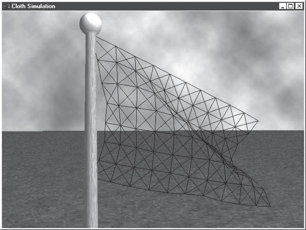
Each line in the wireframe flag shown in Figure 13-1 represents a spring-damper element, while the nodes where these springs intersect represent the particles. We modeled the springs using the spring-damper formulas that we showed you back in Chapter 3. The (initially) horizontal and vertical springs provide the basic structure for the flag, while the diagonal springs are there to resist shear forces and lend further strength to the cloth. Without these shear springs, the cloth would be quite stretchy. Note that there are no particles located at the intersection of the diagonal springs.
In this chapter, we’ll show you how to use those same techniques to simulate something like a hanging rope or vine. You can use these techniques to simulate all sorts of things besides cloth and rope or vines. For example, you can model the swing of a golf club if you can imagine one rigid body representing the arm and another representing the golf club. We’ll get to that example in Chapter 19, but for now let’s see how to model a hanging rope or vine and some other springy objects.
Application of linear springs is not the only method available to connect objects, but it has the advantages of being conceptually simple, easy to implement, and effective. One of the potential disadvantages is that you can run into numerical stability problems if the springs are too stiff. We’ll talk more about these issues throughout this chapter. Also, the examples we’ll cover are in 2D for simplicity, but the techniques apply in 3D, too.
Springs and Dampers
You learned in Chapter 3 that springs are structural elements that, when connected between two objects, apply equal and opposite forces to each object. This spring force follows Hooke’s law and is a function of the stretched or compressed length of the spring relative to the rest length of the spring and the spring constant. The spring constant is a quantity that relates the force exerted by the spring to its deflection:
| Fs = –ks (L – r) |
Here, Fs is the spring force, ks is the spring constant, L is the stretched or compressed length of the spring, and r is the rest length of the spring. The negative sign in the preceding equation just means that the force is in the opposite direction of the displacement.
Dampers are usually used in conjunction with springs in numerical simulations. They act like viscous drag in that dampers act against velocity. The force developed by a damper is proportional to the relative velocity of the connected objects and a damping constant, kd, that relates relative velocity to damping force.
| Fd = –kd (v1 – v2) |
This equation shows the damping force, Fd, as a function of the damping constant and the relative velocity of the connected points on the two connected bodies.
Typically, springs and dampers are combined into a single spring-damper element where a single formula is used to represent the combined force. In vector notation, the formula for a spring-damper element connecting two bodies is:
| F1 = –{ks (L – r) + kd ((v1 – v2) • L)/L} L/L |
Here, F1 is the force exerted on body 1, while the force, F2, exerted on body 2 is:
| F2 = –F1 |
L is the length of the spring-damper (L, not in bold print, is the magnitude of the vector L), which is equal to the vector difference in position between the connected points on bodies 1 and 2. If the connected objects are particles, then L is equal to the position of body 1 minus the position of body 2. Similarly, v1 and v2 are the velocities of the connected points on bodies 1 and 2. The quantity (v1 – v2) represents the relative velocity between the connected bodies.
It’s fairly straightforward to connect particles with springs (and dampers); you need only specify the particles to which the spring is connected and compute the stretched or compressed length of the spring as the particles move relative to each other. The force generated by the spring is then applied equally (but in opposite directions) to the connected particles. This is a linear force.
For rigid bodies, things are a bit more complicated. First, not only do you have to specify to which body the spring is attached, but you must also specify the precise points on each object where the spring attaches. Then, in addition to the linear force applied by the spring to each body, you must also compute the resulting moment on each body causing each to rotate.
Connecting Particles
From swinging vines in Activision’s Pitfall to barnacle tongues in Valve Corporation’s Half-Life, dangling rope-like objects have appeared in video games in various incarnations since the very early days of video gaming. Some implementations, such as those in the 1982 versions of Pitfall, are implemented rather simply and unrealistically, while others, such as barnacle tongues, are implemented more realistically in how they dangle and swing. Whether it’s a vine, rope, chain, or tongue, you can use particles and springs to simulate realistic rope-like behavior. We’ll show you how in the following simple example.
Rope
You know from your real-life experience that ropes are flexible, although some are more flexible than others. Ropes are elastic and stretch to varying extents. They drape when suspended by their two ends. They bend when swinging or when collapsing on the ground. We can capture all these behaviors using simple particles connected with springs. Figure 13-2 illustrates the rope example we’ll cover here.
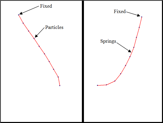
The example consists of a rope comprising 10 particles and 9 springs. At the start of the simulation, the rope, originally extended straight out to the right, falls under the influence of gravity, swinging left and right until it comes to rest (hanging straight down). The dots represent particles and the lines represent springs. The topmost particle is fixed, and the illustration on the left in Figure 13-2 shows the rope swinging down from right to left while the illustration on the right shows the rope swinging back from left to right.
This example uses all the same code and techniques presented in Chapter 7 through Chapter 9 for simulating particles and rigid bodies. Really, the only difference is that we have to compute a new force—the spring force on each object. But before we do that, we have to define and initialize the springs.
Spring structure and variables
The following code sample shows the spring data structure we set up to store each spring’s information:
typedef struct _Spring {
    int        End1;
    int        End2;
    float      k;
    float      d;
    float      InitialLength;
} Spring, *pSpring;
Specifically, this information includes:
End1A reference to the first particle to which the spring is connected
End2A reference to the second particle to which the spring is connected
kThe spring constant
dThe damping constant
InitialLengthThe unstretched length of the spring
This structure is appropriate for connecting particles. We’ll make a slight modification to this structure later, when we get to the example where we’re connecting rigid bodies.
There are defines and
variables unique to this example that must be set up as
follows:
#define        _NUM_OBJECTS     10
#define        _NUM_SPRINGS     9
#define        _SPRING_K        1000
#define        _SPRING_D        100

Particle        Objects[_NUM_OBJECTS];
Spring          Springs[_NUM_SPRINGS];
As stated earlier, there are 10 particles (objects) and 9
springs in this simulation. The arrays Objects and Springs are used to keep track of them. We
also set up a few defines
representing the spring and damping constants. The values shown here
are arbitrary, and you can change them to suit whatever behavior you
desire. The higher the spring constant, the stiffer the springs;
whereas the lower the spring constant, the stretchier the springs.
Stretchy springs make your rope more elastic. Keep in mind while
tuning these values that if you make the spring constant too high,
you’ll probably have to make the simulation time step smaller and/or
use a robust integration scheme to avoid numerical
instabilities.
The damping constant controls how quickly the springiness of the springs dampens out. You’ll end up tuning this value to get the behavior you desire. A small value can make the rope seem jittery, while a large value will make the stretchiness appear smoother. Higher damping also helps alleviate numerical instabilities to some extent, although it’s no substitute for a robust integration scheme.
Initialize the particles and springs
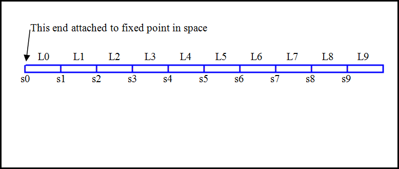
Initially, our particle rope is set up horizontally, as shown in Figure 13-3, with the leftmost particle, p0, fixed—that is, the particle p0 will not move, and the remainder of the rope will pivot about p0. For convenience, all remaining particles are incrementally indexed from left to right.
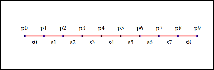
There are nine springs, which are indexed from left to right as illustrated in Figure 13-3. Spring 0 connects particle 0 to particle 1, spring 1 connects particle 1 to particle 2, and so on. The following code sample shows how all this is initialized:
bool    Initialize(void)
{
    Vector    r;
    int       i;

    Objects[0].bLocked = true;

    // Initialize particle locations from left to right.
    for(i=0; i<_NUM_OBJECTS; i++)
    {
        Objects[i].vPosition.x = _WINWIDTH/2 + Objects[0].fLength * i;
        Objects[i].vPosition.y = _WINHEIGHT/8;
    }

    // Initialize springs connecting particles from left to right.
    for(i=0; i<_NUM_SPRINGS; i++)
    {
        Springs[i].End1 = i;
        Springs[i].End2 = i+1;
        r = Objects[i+1].vPosition - Objects[i].vPosition;

        Springs[i].InitialLength = r.Magnitude();
        Springs[i].k = _SPRING_K;
        Springs[i].d = _SPRING_D;
    }
    return true;
}
First, the local variables r
and i are declared. r will be used to compute the initial,
unstretched length of the springs, and i will be used to index the Objects and Springs arrays. Second, Objects[0], the one that is fixed, has its
bLocked property set to true, indicating that it does not move (that
is, it’s locked).
Next, the particle positions are initialized starting from the first particle—the
fixed one positioned at the middle of the screen—and proceeding to the rest of the
particles, offsetting each to the right by an amount equal to property fLength. fLength is an
arbitrary length that you can define, that represents the spacing of the particles and,
subsequently, the initial length of the springs connecting the particles.
Finally, we set up the springs, connecting each particle to its
neighbor on the right. Starting at the first spring, we set its end
references to the index of the particle to its left and right in the
properties End1 and End2, respectively. These indices are simply
i and i+1, as shown in the preceding code sample
within the last for loop. The
initial length vector of the spring is computed and stored in the
vector r, where r = Objects[i+1].vPosition -
Objects[i].vPosition. The magnitude of this vector is the
initial spring length, which is stored in the spring’s property,
InitialLength. This step isn’t
strictly necessary in this example since you already know that the
property fLength discussed earlier
is the initial length of each spring. However, we’ve done it this
general way since you may not necessarily initialize the particle
positions as we have simply done.
Update the simulation
Updating the particle positions at each simulation time step, under the influence of gravity and spring forces
proceeds just like in the earlier examples of Chapter 8 and Chapter 9. Essentially, you must compute the forces on the
particles, integrate the equations of motion, and redraw the scene. As usual in our
examples, the function UpdateSimulation is called on to
perform these tasks. For the current example, UpdateSimulation looks like this:
void    UpdateSimulation(void)
{
    double    dt = _TIMESTEP;
    int       i;
    double    f, dl;
    Vector    pt1, pt2;
    int       j;
    Vector    r;
    Vector    F;
    Vector    v1, v2, vr;

    // Initialize the spring forces on each object to zero.
    for(i=0; i<_NUM_OBJECTS; i++)
    {
        Objects[i].vSprings.x = 0;
        Objects[i].vSprings.y = 0;
        Objects[i].vSprings.z = 0;
    }

    // Calculate all spring forces based on positions of connected objects.
    for(i=0; i<_NUM_SPRINGS; i++)
    {
        j = Springs[i].End1;
        pt1 = Objects[j].vPosition;
        v1 = Objects[j].vVelocity;

        j = Springs[i].End2;
        pt2 = Objects[j].vPosition;
        v2 = Objects[j].vVelocity;

        vr = v2 - v1;
        r = pt2 - pt1;
        dl = r.Magnitude() - Springs[i].InitialLength;
        f = Springs[i].k * dl; // - means compression, + means tension
        r.Normalize();
        F = (r*f) + (Springs[i].d*(vr*r))*r;

        j = Springs[i].End1;
        Objects[j].vSprings += F;

        j = Springs[i].End2;
        Objects[j].vSprings -= F;
    }

    .
    .
    .
    // Integrate equations of motion as usual.
    .
    .
    .
    // Render the scene as usual.
    .
    .
    .
}
As you can see, there are several local variables here. We’ll explain each one as we
get to the code where it’s used. After the local variable declarations, this function’s
first task is to reset the aggregate spring forces on each particle to 0. Each particle
stores the aggregate spring force in the property vSprings, which is a vector. In this example, each particle will have up to
two springs acting on it at any given time.
The next block of code in the for loop computes the springs forces acting
on each particle. There are several steps to this, so we’ll go through
each one. First the loop is set up to step through the list of
springs. Recall that each spring is connected to two particles, so
each step through the loop will compute a spring force and apply it to
two separate particles.
Within the loop, the variable j is used as a convenience to temporarily
store the index that refers to the Object to which the spring is attached. For
each spring j is first set to the
spring’s End1 property. A temporary
variable, pt1, is then set equal to
the position of the Object to which
j refers. Another temporary
variable, v1, is set to the
velocity of the Object to which
j refers. Next, j is set to the index of End2, the other Object to which the current spring is
attached, and that object’s position and velocity are stored in
pt2 and v2, respectively. This sort of temporary
variable use isn’t necessary, of course, but it makes the following
lines of code that compute the spring force more readable in our
opinion.
vr is a vector that stores
the relative velocity between the two ends of the spring. We compute
vr by subtracting v1 from v2. Similarly, r is a vector that stores the relative
distance between the two ends of the spring. We compute r by subtracting pt1 from pt2. The magnitude of r represents the stretched or compressed
length of the spring. The change in spring length is computed and
stored in dl as follows:
dl = r.Magnitude() - Springs[i].InitialLength;
dl will be negative if the
computed length is shorter than the initial length of the spring. This
implies that the spring is in compression and should act to push the
particles away from each other. A positive dl means the spring is in tension and should
act to pull the particles toward each other. The line:
f = Springs[i].k * dl;
computes the corresponding spring force as a function of
dl and the spring constant. Note
that f is a scalar and we have not
yet computed its line of action, although we know it acts along the
line connecting the particles at End1 and End2. That line is represented by r, which we computed earlier. And the spring
force is just f times the unit
vector along r. Since we’re
including damping, we have to use the spring-damper equation for the
total force acting on each particle, which we call the vector F. F is
computed as follows:
F = (r*f) + (Springs[i].d*(vr*r))*r;
The first term on the right side of the equals sign is the
Hooke’s law–based spring force, and the second term is the damping
force. Note here that r is a unit
vector previously computed using the line:
r.Normalize();
Finally, the spring force is applied to each particle connected by the spring. Remember, the force is equal in magnitude but opposite in direction for each particle. The lines:
        j = Springs[i].End1;
        Objects[j].vSprings += F;
apply the spring force to the particle at the first end of the spring, whereas the lines:
        j = Springs[i].End2;
        Objects[j].vSprings -= F;
apply the opposite spring force to the particle at the second end of the spring.
That’s it for computing and applying the spring forces. The remainder of the code is business as usual, where we compute the force due to gravity and add it to the aggregate spring force for each particle and then integrate the equations of motion. Finally, we render the scene at each time step.
Connecting Rigid Bodies
As with particles, you can connect rigid bodies with springs to simulate some interesting things. For example, you may want to simulate something as simple as a linked chain, where each link is connected to the other in series. Or perhaps you want to simulate connected body parts to simulate rag doll physics or maybe a golfer’s swing. All these require some means of connecting rigid bodies. In this section we’ll show you how to use linear spring-dampers, the same we’ve discussed already, to connect rigid bodies. We’ll start with a simple analog to the rope example discussed earlier. Instead of connecting particles with springs to simulate a dangling rope, we’ll connect rigid links to simulate a dangling rope or chain. Later, we’ll show you how linear springs can be used to restrain angular motion.
Links
In this example, each link is rigid in that it does not deform; however, the links are connected by springs in a way that allows the ensemble to swing, stretch, and bend in a manner similar to a hanging chain. Figure 13-4 illustrates our swinging linked chain as it swings from right to left and then back toward the right.
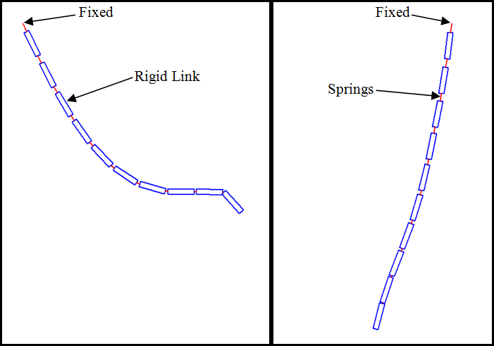
As in the rope example, the topmost link is connected to a fixed point by a spring, such that the linked chain pivots around and hangs from the fixed point. The rectangles represent each rigid link, with the lines connecting the rectangles representing springs.
To model this linked chain, we need only make a few changes to the rope example to address the fact that we’re now dealing with rigid bodies that can rotate versus particles. This requires us to specify the point on each body to which the springs are attached, and in addition to computing the spring forces acting on each body, we must also compute the moments due to those forces. Aside from these spring force and moment computations, the remainder of the simulation is the same as those discussed in Chapter 7 through Chapter 12.
Basic structures and variables
We can use the Spring
structure shown earlier in the rope example again here with one small
modification. Basically, we need to change the type of the endpoint
references, End1 and End2, from integers to a new structure we’ll
call EndPoint. The new Spring structure looks like this:
typedef struct _Spring {
    EndPoint    End1;
    EndPoint    End2;
    float        k;
    float        d;
    float        InitialLength;
} Spring, *pSpring;
The new EndPoint structure is
as follows:
typedef struct _EndPointRef {
    int       ref;
    Vector    pt;
} EndPoint;
Here, ref is the index
referring to the Object to which
the spring is attached, and pt is
the point in the attached Object’s
local coordinate system to which the spring is attached. Notice from
Figure 13-4 that the first spring, the topmost
one, is connected to a single object; the other end of it is connected
to a fixed point in space. We’ll use a ref of −1
to indicate that a spring’s endpoint is connected to a fixed point in
space instead of an object.
As in the rope example, we have a few important defines and variables to set up:
#define        _NUM_OBJECTS     10
#define        _NUM_SPRINGS     10
#define        _SPRING_K        1000
#define        _SPRING_D        100

RigidBody2D       Objects[_NUM_OBJECTS];
Spring            Springs[_NUM_SPRINGS];
These are the same as before except now we have 10 springs
instead of 9, and Objects is of
type RigidBody2D instead of
Particle.
The damping and spring constants play the same role here as they did in the rope example.
Initialize
Initially our linked chain is set up horizontally, just like the rope example, but with the link and spring indices shown in Figure 13-5. Each rectangle represents a rigid link, and a spring attached to the left end of each link connects the link to its neighbor to the left. In the case of the first link, L0, the spring connects the left end of the link to a fixed point in space.
The code for this setup is only a little more involved than that
for the rope example; the additional complexity is due to having to
deal with specific points on the rigid bodies to which each spring is
attached. The following code sample contains the modified Initialize function:
bool    Initialize(void)
{
    Vector    r;
    Vector    pt;
    int       i;

    // Initialize objects for linked chain.
    for(i=0; i<_NUM_LINKS; i++)
    {
        Objects[i].vPosition.x = _WINWIDTH/2 + Objects[0].fLength * i;
        Objects[i].vPosition.y = _WINHEIGHT/8;
        Objects[i].fOrientation = 0;
    }

    // Connect end of the first object to a fixed point in space.
    Springs[0].End1.ref = −1;
    Springs[0].End1.pt.x = _WINWIDTH/2-Objects[0].fLength/2;
    Springs[0].End1.pt.y = _WINHEIGHT/8;

    Springs[0].End2.ref = 0;
    Springs[0].End2.pt.x = -Objects[0].fLength/2;
    Springs[0].End2.pt.y = 0;

    pt = VRotate2D(Objects[0].fOrientation, Springs[0].End2.pt)
         + Objects[0].vPosition;
    r = pt - Springs[0].End1.pt;

    Springs[0].InitialLength = r.Magnitude();
    Springs[0].k = _SPRING_K;
    Springs[0].d = _SPRING_D;

    // Connect end of all remaining springs.
    for(i=1; i<_NUM_LINKS; i++)
    {
        Springs[i].End1.ref = i-1;
        Springs[i].End1.pt.x = Objects[i-1].fLength/2;
        Springs[i].End1.pt.y = 0;

        Springs[i].End2.ref = i;
        Springs[i].End2.pt.x = -Objects[i].fLength/2;
        Springs[i].End2.pt.y = 0;

        pt = VRotate2D(Objects[i].fOrientation, Springs[i].End2.pt)
              + Objects[i].vPosition;
        r = pt - (VRotate2D(Objects[i-1].fOrientation, Springs[i].End1.pt)
                  + Objects[i-1].vPosition);

        Springs[i].InitialLength = r.Magnitude();
        Springs[i].k = _SPRING_K;
        Springs[i].d = _SPRING_D;
    }

    return true;
}
The local variables r and
i are the same as before; however,
there’s a new variable, pt, that we
use to temporarily store the coordinates of specific points when
converting from one coordinate system to another. We’ll see how this
is done shortly.
After the local variables are declared, the Object positions are initialized, starting
from the first Object positioned at
the middle of the screen and proceeding to the rest of the Objects, offsetting each to the right by an
amount equal to property fLength.
Here, fLength is an arbitrary
length representing the length of each rigid body, not the length of
the springs connecting each rigid body. As you’ll see momentarily, the
initial length of all the springs in this example is 0.
You should be aware that the coordinates for each object computed here are the coordinates of the object’s center of gravity, which in this example we defined as the middle of the rectangle representing each object. Since these are rigid bodies, not only must you specify their initial positions, but you must also specify their initial orientations as shown in the preceding code sample. The way we have this example set up, each object is initialized with an orientation of 0 degrees.
The next task is to set up the spring connecting the first link, the one on the left, to a fixed point in space. The following code handles this task:
    // Connect end of the first object to a fixed point in space.
    Springs[0].End1.ref = −1;
    Springs[0].End1.pt.x = _WINWIDTH/2-Objects[0].fLength/2;
    Springs[0].End1.pt.y = _WINHEIGHT/8;

    Springs[0].End2.ref = 0;
    Springs[0].End2.pt.x = -Objects[0].fLength/2;
    Springs[0].End2.pt.y = 0;

    pt = VRotate2D(Objects[0].fOrientation, Springs[0].End2.pt)
         + Objects[0].vPosition;
    r = pt - Springs[0].End1.pt;

    Springs[0].InitialLength = r.Magnitude();
    Springs[0].k = _SPRING_K;
    Springs[0].d = _SPRING_D;
The first spring, Spring[0],
has its first endpoint, End1, set
to refer to −1, which, as explained
earlier, means that this end of the spring is connected to some fixed
point in space. The location of the point, stored in the End1.pt property, must be specified in
global coordinates as shown previously.
Now the second end of the first spring is connected to the left
end of the first link; therefore, End2.ref of the first spring is set to
0, which is the index to the first
Object. The point on Object[0] to which the spring is attached is
the leftmost end on the centerline of the object; thus, its
coordinates—relative to the object’s center of gravity location and
specified in local, body-fixed coordinates—are:
    Springs[0].End2.pt.x = -Objects[0].fLength/2;
    Springs[0].End2.pt.y = 0;
Now remember, the points on Objects to which springs are attached are
specified in body-fixed, local coordinates of each referenced object,
whereas any point fixed in space to which a spring is attached and not
on an Object must be specified in
global, earth-fixed coordinates. You have to keep these coordinates
straight and make the appropriate rotations when computing spring
lengths throughout the simulation. The code;
    pt = VRotate2D(Objects[0].fOrientation, Springs[0].End2.pt)
         + Objects[0].vPosition;
    r = pt - Springs[0].End1.pt;
illustrates how to do this. To compute the initial spring
length, we need to compute the relative distance between the endpoints
of the spring. In case of the first spring, End1 was specified in global coordinates,
but End2 was specified in the local
coordinate system of Object[0].
Therefore, we have to convert the coordinates of End2 from local coordinates to global
coordinates before calculating the relative distance between the ends.
The preceding line, which calls the VRotate2D function you saw in earlier
chapters, rotates the locally specified point, End2.pt, from local to global coordinates;
it then adds the Object’s position
to the result, arriving at a point, pt, in global coordinates coincident with
the second endpoint of the spring. The relative distance, r, is the second endpoint, pt, minus the first endpoint, End1.pt.
Finally, we compute the initial length of the spring by taking
the magnitude of r and storing the
result in the spring’s InitialLength property.
With the first spring out of the way, the Initialize function enters a loop to set up
the remaining springs. Proceeding from left to right in Figure 13-5, the first endpoint, End1, is connected to the right side of
Object[i-1], and the second
endpoint, End2, is connected to the
left side of Object[i]. Be aware
that each endpoint of each spring is specified in different coordinate
systems. The left end is in the coordinate system of Object[i-1], while the right end is in the
coordinate system of Object[i]. It
may seem trivial during this setup, but when things start moving and
rotating it is critically important to keep these coordinate systems
straight. Doing so involves transforming each endpoint coordinate from
the local system of the body to which it’s attached to the global
coordinate system. This is illustrated as follows:
        pt = VRotate2D(Objects[i].fOrientation, Springs[i].End2.pt)
              + Objects[i].vPosition;
        r = pt - (VRotate2D(Objects[i-1].fOrientation, Springs[i].End1.pt)
                  + Objects[i-1].vPosition);
The first line converts the spring attachment point End2 from the local coordinate system of
Object[i] to global coordinates by
performing a rotation and translation using functions you’ve already
seen numerous times now. The result is temporarily stored in the local
variable, pt. The second line
converts the spring attachment point End1 from the local coordinate system of
Object[i-1] to global coordinates
and then subtracts the result from pt, yielding a vector, r, representing the relative distance
between the spring’s endpoints. The magnitude of r is the spring’s initial length. Performing
these same calculations during the simulation will result in the
spring’s stretched or compressed length. That calculation is performed
in UpdateSimulation.
Update
The function UpdateSimulation
is substantially the same as that discussed in the rope example. There
are a few differences that we’ll highlight here. Again, these
differences are due to the fact that we’re now dealing with rigid
bodies that rotate rather than simple particles. The following code
sample shows the additions to UpdateSimulation. You can see there are a
couple of new variables, M and
Fo. M is used to temporarily store moments due
to spring forces Fo in the local
coordinates of each Object.
Just as the property vSprings was initialized to 0
at the start of UpdateSimulation, so too must we
initialize vMSprings to 0. Recall, vSprings aggregates the spring forces acting on each Object. For rigid bodies that rotate, we’ll use vMSprings to aggregate the moments on each Object resulting from those spring forces:
void    UpdateSimulation(void)
{
    .
    .
    .
    Vector    M;
    Vector    Fo;

    // Initialize the spring forces and moments on each object to zero.
    for(i=0; i<_NUM_OBJECTS; i++)
    {
        .
        .
        .

        Objects[i].vMSprings.x = 0;
        Objects[i].vMSprings.y = 0;
        Objects[i].vMSprings.z = 0;
    }

    // Calculate all spring forces based on positions of connected objects
    for(i=0; i<_NUM_SPRINGS; i++)
    {
        if(Springs[i].End1.ref == −1)
        {
            pt1 = Springs[i].End1.pt;
            v1.x = v1.y = v1.z = 0; // point is not moving
        } else {
            j = Springs[i].End1.ref;
            pt1 = Objects[j].vPosition + VRotate2D(Objects[j].fOrientation,
                                                   Springs[i].End1.pt);
            v1 = Objects[j].vVelocity + VRotate2D(Objects[j].fOrientation,
                 Objects[j].vAngularVelocity^Springs[i].End1.pt);
        }

        if(Springs[i].End2.ref == −1)
        {
            pt2 = Springs[i].End2.pt;
            v2.x = v2.y = v2.z = 0;
        } else {
            j = Springs[i].End2.ref;
            pt2 = Objects[j].vPosition + VRotate2D(Objects[j].fOrientation,
                                                   Springs[i].End2.pt);
            v2 = Objects[j].vVelocity + VRotate2D(Objects[j].fOrientation,
                 Objects[j].vAngularVelocity^Springs[i].End2.pt);
        }

        // Compute spring-damper force.
        vr = v2 - v1;
        r = pt2 - pt1;
        dl = r.Magnitude() - Springs[i].InitialLength;
        f = Springs[i].k * dl;
        r.Normalize();
        F = (r*f) + (Springs[i].d*(vr*r))*r;

        // Aggregate the spring force on each connected object
        j = Springs[i].End1.ref;
        if(j != −1)
            Objects[j].vSprings += F;

        j = Springs[i].End2.ref;
        if(j != −1)
            Objects[j].vSprings −= F;


        // convert force to first ref local coords
        // Get local lever
        // calc moment

        // Compute and aggregate moments due to spring force
        // on each connected object.
        j = Springs[i].End1.ref;
        if(j != −1)
        {
            Fo = VRotate2D(-Objects[j].fOrientation, F);
            r = Springs[i].End1.pt;
            M = r^Fo;
            Objects[j].vMSprings += M;
        }

        j = Springs[i].End2.ref;
        if(j!= −1)
        {
            Fo = VRotate2D(-Objects[j].fOrientation, F);
            r = Springs[i].End2.pt;
            M = r^Fo;
            Objects[j].vMSprings −= M;
        }
    }
    .
    .
    .
    // Integrate equations of motion as usual.
    .
    .
    .
    // Render the scene as usual.
    .
    .
    .
}
As in the rope example, UpdateSimulation steps through all the
Springs, computing their stretched
or compressed length, the relative velocity of each spring’s
endpoints, and the resulting spring forces. These calculations are a
bit different in this current example because we have to handle
rotation, as explained earlier.
Upon entering the for loop in
the preceding code sample, End1 of
the current spring is checked to see if it’s connected to a fixed
point in space. If so, the temporary variable pt1 stores the global coordinates of the
endpoint, and the variable v1
stores the velocity of the endpoint, which is 0. If the endpoint
reference is a valid Object, then
we compute the position of the endpoint, stored in pt1, just like we did in the Initialize function, using a coordinate
transform as follows:
pt1 = Objects[j].vPosition + VRotate2D(Objects[j].fOrientation,
                                       Springs[i].End1.pt);
We compute the velocity of that point as shown in Chapter 9 by first computing the velocity of
the point due to rotation in body-fixed coordinates, converting that
to global coordinates, and then adding the result to the Object’s linear velocity. This is accomplished in the following
code:
v1 = Objects[j].vVelocity + VRotate2D(Objects[j].fOrientation,
     Objects[j].vAngularVelocity^Springs[i].End1.pt);
We then repeat these calculations for the second endpoint of the spring.
Once we’ve obtained the positions and velocities of the spring
endpoints, we compute the spring-damper force in the same manner as in
the rope example. The resulting spring forces are aggregated in the
vSprings property of each object.
Note that if the spring endpoint reference is a fixed point in space,
we do not aggregate the force on that fixed point.
Since the Objects are rigid
bodies here, we now have to compute the moment due to the spring force
acting on each object. You must do this so that when we integrate the
equations of motion, the objects rotate properly.
For the Object connected to
End1 of the current spring, the
following lines compute the moment:
            Fo = VRotate2D(-Objects[j].fOrientation, F);
            r = Springs[i].End1.pt;
            M = r^Fo;
            Objects[j].vMSprings += M;
Fo is a vector representing
the spring force computed earlier on the current Object in the current Object’s local, body-fixed coordinate
system. The line:
Fo = VRotate2D(-Objects[j].fOrientation, F);
transforms F from global to
local coordinates of the current Object, Object[j].
r is set to the local,
body-fixed coordinates of the spring attachment point for the current
Object, and we compute the
resulting moment by taking the vector cross product of r with Fo. The result is stored in the vector
variable M, which gets aggregated
in the Object property vMSprings. We then perform these same sorts
of calculations for the Object
connected to the other end of the spring.
After these calculations, the rest of UpdateSimulation is the same as that shown
earlier; the function integrates the equations of motion and renders
the scene.
Upon running this simulation, you’ll see the linked chain swing down and to the left and then back and forth until the motion dampens out. You’ll also notice there’s some stretch to the springs between the objects that appears to increase as you look from the lower link to the upper link. This is indeed a non-uniform stretch in the springs, which makes sense when you consider that the upper spring has more weight, thus more force, pulling down on it than does the lower spring.
As in this rope example, you can tune the spring and damping constants to minimize the spring stretch if that gap created by the stretched spring bothers you. You must keep in mind numerical stability if your springs are too stiff, and here again, you must implement a robust integrator.
Rotational Restraint
So far we’ve used springs only to attach objects in a way that keeps the attachment points together but allows the objects to rotate about the attachment point. This is a so-called pinned joint. If you want a fixed joint that minimizes the amount of rotation between the connected objects, you can add another spring to restrain the connected objects’ rotation.
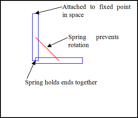
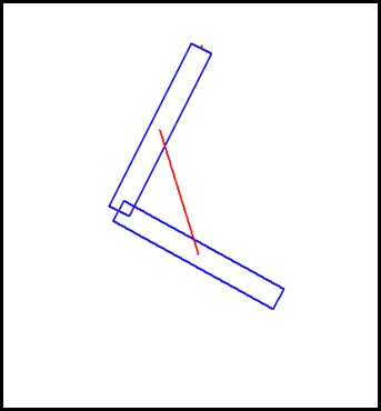
Figure 13-6 illustrates an example comprising two rigid objects connected at their ends, forming a ninety-degree angle. The uppermost end of the first object is connected to a fixed point in space as in our rope and linked-chain examples. Under gravity, the assembly would rotate and swing around this fixed point. However, unlike the linked-chain example, the extra spring prevents the lower link from pivoting around the other end of the first link, as illustrated in Figure 13-7.
The setup for this example is relatively straightforward and consists of setting the initial positions and orientations of two rigid bodies and connecting three springs.
This example’s Initialize
function is as follows:
bool    Initialize(void)
{
    Vector    r;
    Vector    pt;
    int       i;

    // Position objects
    Objects[0].vPosition.x = _WINWIDTH/2;
    Objects[0].vPosition.y = _WINHEIGHT/8+Objects[0].fLength/2;
    Objects[0].fOrientation = 90;

    Objects[1].vPosition.x = _WINWIDTH/2+Objects[1].fLength/2;
    Objects[1].vPosition.y = _WINHEIGHT/8+Objects[0].fLength;
    Objects[1].fOrientation = 0;

    // Connect end of the first object to the earth:
    Springs[0].End1.ref = −1;
    Springs[0].End1.pt.x = _WINWIDTH/2;
    Springs[0].End1.pt.y = _WINHEIGHT/8;

    Springs[0].End2.ref = 0;
    Springs[0].End2.pt.x = -Objects[0].fLength/2;
    Springs[0].End2.pt.y = 0;

    pt = VRotate2D(Objects[0].fOrientation, Springs[0].End2.pt) +
         Objects[0].vPosition;
    r = pt - Springs[0].End1.pt;

    Springs[0].InitialLength = r.Magnitude();
    Springs[0].k = _SPRING_K;
    Springs[0].d = _SPRING_D;

    // Connect other end of first object to end of second object
    i = 1;
    Springs[i].End1.ref = i-1;
    Springs[i].End1.pt.x = Objects[i-1].fLength/2;
    Springs[i].End1.pt.y = 0;

    Springs[i].End2.ref = i;
    Springs[i].End2.pt.x = -Objects[i].fLength/2;
    Springs[i].End2.pt.y = 0;

    pt = VRotate2D(Objects[i].fOrientation, Springs[i].End2.pt) +
         Objects[i].vPosition;
    r = pt - (VRotate2D(Objects[i-1].fOrientation, Springs[i].End1.pt) +
              Objects[i-1].vPosition);

    Springs[i].InitialLength = r.Magnitude();
    Springs[i].k = _SPRING_K;
    Springs[i].d = _SPRING_D;

    // Connect CG of objects to each other
    Springs[2].End1.ref = 0;
    Springs[2].End1.pt.x = 0;
    Springs[2].End1.pt.y = 0;

    Springs[2].End2.ref = 1;
    Springs[2].End2.pt.x = 0;
    Springs[2].End2.pt.y = 0;

    r = Objects[1].vPosition - Objects[0].vPosition;

    Springs[2].InitialLength = r.Magnitude();
    Springs[2].k = _SPRING_K;
    Springs[2].d = _SPRING_D;
}
The two Objects are positioned
with the lines:
    Objects[0].vPosition.x = _WINWIDTH/2;
    Objects[0].vPosition.y = _WINHEIGHT/8+Objects[0].fLength/2;
    Objects[0].fOrientation = 90;

    Objects[1].vPosition.x = _WINWIDTH/2+Objects[1].fLength/2;
    Objects[1].vPosition.y = _WINHEIGHT/8+Objects[0].fLength;
    Objects[1].fOrientation = 0;
Basically, the first Object,
Object[0], is located somewhere
toward the top middle of the screen with an initial rotation of ninety
degrees so that it stands vertically. The second Object, Object[1], is positioned so that it lies
horizontally with its left end coincident with the lower end of the
first object. We’ll put a spring there momentarily, but first, we’ll
connect a spring to the upper end of the first object to connect it to a
fixed point. The following code takes care of that spring using the same
techniques discussed earlier:
    // Connect end of the first object to the earth:
    Springs[0].End1.ref = −1;
    Springs[0].End1.pt.x = _WINWIDTH/2;
    Springs[0].End1.pt.y = _WINHEIGHT/8;

    Springs[0].End2.ref = 0;
    Springs[0].End2.pt.x = -Objects[0].fLength/2;
    Springs[0].End2.pt.y = 0;

    pt = VRotate2D(Objects[0].fOrientation, Springs[0].End2.pt) +
         Objects[0].vPosition;
    r = pt - Springs[0].End1.pt;

    Springs[0].InitialLength = r.Magnitude();
    Springs[0].k = _SPRING_K;
    Springs[0].d = _SPRING_D;
Now, we connect a spring at the corner formed by the two objects using the following code:
    // Connect other end of first object to end of second object
    i = 1;
    Springs[i].End1.ref = i-1;
    Springs[i].End1.pt.x = Objects[i-1].fLength/2;
    Springs[i].End1.pt.y = 0;

    Springs[i].End2.ref = i;
    Springs[i].End2.pt.x = -Objects[i].fLength/2;
    Springs[i].End2.pt.y = 0;

    pt = VRotate2D(Objects[i].fOrientation, Springs[i].End2.pt) +
         Objects[i].vPosition;
    r = pt - (VRotate2D(Objects[i-1].fOrientation, Springs[i].End1.pt) +
              Objects[i-1].vPosition);

    Springs[i].InitialLength = r.Magnitude();
    Springs[i].k = _SPRING_K;
    Springs[i].d = _SPRING_D;
If we stop here, the simulation will behave just like the linked-chain example, albeit we’ll have a very short chain. So, to prevent rotation at the corner, we’ll add another spring connecting the centers of gravity of the objects. You can use other points if you desire; we chose the centers of gravity for convenience. The following code adds this rotational restraint spring:
    // Connect CG of objects to each other
    Springs[2].End1.ref = 0;
    Springs[2].End1.pt.x = 0;
    Springs[2].End1.pt.y = 0;

    Springs[2].End2.ref = 1;
    Springs[2].End2.pt.x = 0;
    Springs[2].End2.pt.y = 0;

    r = Objects[1].vPosition - Objects[0].vPosition;

    Springs[2].InitialLength = r.Magnitude();
    Springs[2].k = _SPRING_K;
    Springs[2].d = _SPRING_D;
The rest of this simulation is the same as in the linked-chain example. There are no other code modifications required. It’s all in the setup.
Now, if you want to allow some amount of rotation or flexibility in the joint, you can do so by tuning the spring constant for the rotation restraint spring. Using linear springs creatively, you can model all sorts of joints very simply.