
Chapter 22. Gaming from One Place to Another
Once a tool meant to help the United States guide intercontinental ballistic missiles, the Global Positioning System (GPS) has evolved to be a part of our everyday lives. The current generation will never have known a world where getting lost was something that couldn’t be fixed by trilaterating their position between satellites orbiting the planet. Although GPS has become commonplace in the navigational world, the proliferation of smartphones is just now opening the doors to GPS gaming. While this genre is just emerging, we’d like to give you an introduction to the physics behind GPS and the current applications in the gaming world.
Let’s recall that positions near the earth’s surface are generally given in the geographic coordinate system, more often described as latitude, longitude, and altitude. Latitude is a measure in degrees of how far north or south you are from the equator. Longitude is the measure in degrees of how far east or west you are from the prime meridian. A meridian is a line of constant latitude that runs from the North Pole to the South Pole. The prime meridian is arbitrarily defined as the meridian that passes through the Greenwich Observatory in the UK. Altitude is usually given as the measure of how far above or below sea level you are at the point described by latitude and longitude.
Location-Based Gaming
Before getting to the physics behind GPS, we’d like to take a moment to discuss how GPS is being implemented into games. Right now, this is an emerging market that is just starting to gain traction. There are several broad categories into which games fall. Another step beyond what the accelerometer did, GPS enables users to move computer games not only off the couch but also out into the world.
Geocaching and Reverse Geocaching
Geocaching is the oldest form of gaming involving GPS. It originated after selective availability was removed from GPS, making it more accurate, in the year 2000. In its most basic form, it is the process of hunting down a “cache” using provided GPS coordinates. The cache usually has a logbook and may contain other items such as coins with serial numbers that the finder can move to another cache and track online.
Because of the large amount of setup involved in implementing a geocaching game on a commercial scale, most implementations are community based. However, reverse geocaching has more promise for the gaming industry. In this variation there is nothing at the supplied coordinates, but traveling to them is required to execute some action. Think of it as carrying around a cache that cannot be unlocked until it is within range of some specific coordinate. This could be used to force users to travel in order to unlock a game item. For instance, perhaps to gain the ability to use a sword in a game, the user must travel to the nearest sporting goods store. The commercial possibility of corporate tie-ins is an obvious plus.
Mixed Reality
Mixed-reality games are similar to geocaching. They go beyond just using the coordinates of the user to trigger events, to using reality-based locals. A current example is Gbanga’s Famiglia. In this game your movement in the real world allows you to discover virtual establishments in the game world. This divorces it from the actual physical locations that your GPS is reporting but requires moving between locations in the real world to move your character in the virtual world. Popular right now is the FourSquare app on mobile devices. This is the simplest possible implementation of mixed-reality gaming. FourSquare allows a user to become the mayor of a place if she “checks in” at the locale more than anyone else.
Street Games
Street games are another step beyond mixed reality. These turn the environment around the user into a virtual game board. One example is the recent Pac-Manhattan multiplayer game using GPS in smartphones to play a live version of Pac-Man in Washington Square Park. In general, the idea is to create a court for game play using the environment surrounding the user. The relationship between users is tracked in the virtual space of the game and provides the interactive elements.
What Time Is It?
The story of GPS really begins with a prize offered by the British government in 1717 for a simple way to determine your longitude. Awarded in 1773, the accepted solution was to compare local noon to the official noon sighted at the Greenwich Observatory. The difference between these two times would allow you to tell how far around the world you were from the observatory. Fast-forward three centuries, and we have satellites orbiting the earth, broadcasting time-stamped messages. By calculating the difference between the time the message was received and the time it was transmitted, we can calculate our distance from the satellite. In both cases you need an accurate way to keep or measure time. For sailors in the 1800s, the device was the newly invented chronometer. For us, it is the atomic clock.
Because the signals from a GPS satellite are moving at the speed of light, you need a very accurate clock to keep track of how long it took to travel to you. For instance, if the clock you are using to time when the signal arrives is 1 microsecond off, you will estimate a distance over 900 miles in error. On the supply side of the signal, each satellite has an atomic clock, and internal GPS time is accurate to about 14 nanoseconds. The problem is that you also need a very accurate clock in the receiver, and it would be pretty hard to fit an atomic clock into a phone economically. To get around this, the receiver must figure out the correct current time based on the signals from the satellites.
Two-Dimensional Mathematical Treatment
This section will give you a good idea of how GPS systems determine their location. This background will help you in many applications of geometry in games in general, but most GPS devices do the heavy lifting and report through an API your current latitude and longitude. Some APIs may include more information—for example, the current iOS API, called Core Location, gives the current latitude and longitude, the direction of travel, the distance traveled, and the distance in meters to a given coordinate. It also gives an estimate for the error associated with its position fix in meters.
One way to get your position via the kind of information that GPS provides is a technique called trilateration. We are going to give this problem a mathematical treatment in two dimensions. You could extend this to three dimensions by using spheres instead of circles.
To begin, we can list our unknowns: our x coordinate and y coordinate in space, and the error in our receiver’s clock (or bias), b. In a two-dimensional plane, trilateration among three circles gives you an exact position; in three-dimensional space, four spheres are required to determine all three special coordinates. Note that if we included an assumption about being on the surface of some geometric shape, such as the earth, we could reduce the number of unknowns. No such simplification is used here to provide you with the most general case.
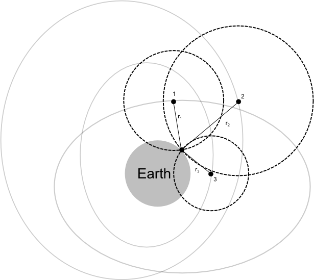
In our example, we are somewhere on the surface of the two-dimensional earth, shown in Figure 22-1 as a light gray solid disk. This disk is being orbited by several GPS satellites. The satellites’ orbits are regular, and their positions at any time are tabulated in an almanac that is stored in the receiver. The time of transmission is encoded in the signal so that the givens are xi, yi, and ti, with i =1,2,3.
To make things easier for us, we are going to abandon the coordinate system of the earth and use the coordinate system defined by our three satellites. The origin will be at satellite 1, the x-axis going directly from satellite 1 straight to satellite 2 and the y-axis being perpendicular to that. This is shown in Figure 22-2.
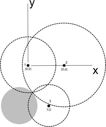
The equations of the three circles are therefore:
| r21 = x2+y2 |
| r22 = (x–d)2+y2 |
| r23 = (x–i)2+(y–j)2 |
Each radius is found by subtracting the transmission time, ti, from the current time and multiplying by the speed of light. As the speed of light is very large, and our current time is only a rough estimate, these radii are commonly referred to as pseudoranges to remind us they are still approximate. The x and y values that satisfy these equations are our current location in two-dimensional space. We now subtract the second equation from the first:
| r12 – r22 = x2 + y2 – (x-d)2 – y2 |
| r12 – r22 = x2 – (x-d)2 |
Solving for x gives:
| x = (r12 – r22+d2) / 2d |
where d is the distance between the known locations of satellite 1 and satellite 2. We now substitute our x coordinate back into the first circle’s equation:
| y2 = r12 – [((r12 – r22 + d2)2) / (4d2)] |
and finally after we take the square root:
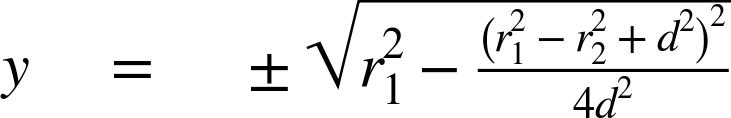
notice that the y value is now expressed as a positive or negative square root. This means there can be zero, one, or two real-number solutions. If the circles do not intersect, then the quantity under the square root will be negative and the y value will have zero real solutions. This is unlikely for the first two satellites because you have already received pseudoranges to them in the form of r1 and r2, which the algorithm assumes to have zero error. If the two circles happen to intersect at only a single tangent point, the y will have one solution and will be equal to 0. This is also unlikely. The most likely result will be that y will be the set of two values, plus or minus the square root of a positive value, and that those two points will be widely separated.
Now if we included the assumption that we were on the earth’s surface, we could already break the tie between the two points by picking whichever was closest to the earth’s surface. However, we still would have to deal with the likelihood that there is a large error in our position given the imprecise clock in the receiver.
We can fix our position (x,y) with no assumptions and account for clock bias by introducing the third point and its pseudorange. Now, it was very likely that the circles obtained from the first two satellites would intersect because of the way that GPS satellites are arranged around the earth. However, because our calculations use pseudoranges, it is relatively unlikely that the third circle will pass directly through one of the two points defined by the intersection of the first two circles. To remove such clock-related distance errors, we first calculate which point (x,y) or (x,–y) is closer to (i,j) and choose that to be our assumed location. The difference between the smaller of these two distances and the pseudorange r3 is then our distance correction, da. As the signal is traveling at the speed of light, the following quotient provides an estimate of the error between the correct time and the receiver’s time:
| b = da/c |
As all the GPS satellites have synchronized atomic clocks, the same bias exists for each. This means that the bias we calculated would actually affect the first pseudoranges we used to find our initial bias. Therefore an iterative approach is required to adjust all the variables in real time until they converge. A more direct, but less obvious, algebraic solution that requires no iteration was developed by Stephen Bancroft. It is detailed in his paper “An Algebraic Solution of the GPS Equations” in the IEEE Transactions on Aerospace and Electronics Systems journal.
Besides clock errors, other errors are introduced by the atmosphere, signals bouncing off the ground and back to the receiver, relativistic effects (discussed in Chapter 2), and atomic clock drift. These are all accounted for in mathematical models applied to the raw position data. For instance, the GPS clocks lose about 7,214 nanoseconds every day due to their velocity according to special relativity. However, because they are higher up in the earth’s gravity well, they gain 45,850 nanoseconds every day according to general relativity. The net effect is found by adding these values together: they run 38,640 nanoseconds faster each day, which would cause about 10 kilometers inaccuracy to build each day they are in orbit. To account for this, the clocks in the GPS receivers are pre-adjusted from 10.23 MHz to 10.22999999543 MHz. The fact that we are giving you a number to 11 decimal places demonstrates the amount of accuracy the modern age enjoys in its time keeping.
Once the bias is taken care of and all the other possible errors adjusted for, the converged solution can be translated back into whatever coordinate system is convenient to give to the end user. Usually this is latitude, longitude, and altitude. Next, we will learn how to calculate different quantities based in the geographic coordinate system.
Location, Location, Location
Let’s take a minute to discuss distance between two latitude and longitude coordinates. You might be tempted to calculate it as the distance between two points. For very small distances, this approximation is probably accurate enough. However, because the earth is actually a sphere, over great distances the calculated route will be much shorter than the actual distance along the surface.
The shortest distance between two points on a sphere, especially in problems of navigation, is called a great circle. A great circle is the intersection of a sphere and a plane defined by the center point of the sphere, the origin, and the destination. The resulting course actually has a heading that constantly changes. On ships, this is avoided in favor of using a rhumb line, which is the shortest path of constant heading. This makes navigation easier at the expense of time. Airplanes, however, do follow great-circle routes to minimize fuel burn.
Distance
There are several ways of calculating the distance along a great circle. The one we will discuss here is the haversine formula. There are other methods like the spherical law of cosines and the Vincenty formula, but the haversine is more accurate for small distances than the spherical law of cosines while remaining much simpler than the Vincenty formula.
The haversine formula for distance is:
| d = (R)(c) |
where R = earth’s radius and c is the angular distance in radians given by:
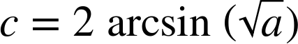
Here, a is the square of half the chord length between the two points, calculated as:
| a = sin2(Δlat/2) + cos(lat1)cos(lat2)sin2(Δlong /2) |
Finally:
| Δlong = long2 – long1 |
| Δlat = lat2 – lat1 |
Remember to first convert the angles to radians before using them in the trig function. Next we will begin showing you an implementation of several different formulas in Objective-C; however, these should translate to C with little modification. These all use the following data structure to hold latitude and longitude information:
typedef enum {
float lat;
float lon;
} Coordinate2D;
Given this, the haversine implementation would look like:
float distanceGreatCircle(Coordinate2D startPoint, Coordinate2D endPoint){

    //Convert location from degrees to radians
    float lat1 = (M_PI/180.) * startPoint.lat;
    float lon1 = (M_PI/180.) * endPoint.longi;
    float lat2 = (M_PI/180.) * endPoint.lat;
    float lon2 = (M_PI/180.) * endPoint.longi;

    //Calculate deltas
float dLat = lat2 - lat1;
    float dLon = lon2 - lon1;

    //Calculate half chord legnth
float a = sin(dLat/2) * sin(dLat/2) + cos(lat1) * cos(lat2) * sin(dLon/2)
                                                           * sin(dLon/2);

//Calculate angular distance
    float C = 2 * atan(sqrt(a)/sqrt(1-a));

//Find arclength
    float distance = 6371 * C; //6371 is radius of earth in km
    return distance;
}
One limitation of the preceding method is that if the two locations are nearly antipodal—that is, on opposite sides of the earth—then the haversine formula may have round-off issues that could results in errors on the order of 2 km. These, however, will be over a distance of 20,000 km. If extreme accuracy is required for nearly antipodal coordinates, you can fall back to the spherical law of cosines, which is best suited for large distances such as the antipodal case.
Great-Circle Heading
As discussed before, to follow the shortest path between two points on a sphere you must travel along a great circle. However, this requires that your heading be constantly changing with time. The formula to calculate your initial heading, or forward azimuth, is:
| Θi = atan2[sin(Δlong)cos(lat2), cos(lat1)sin(lat2) – sin(lat1)cos(lat2)cos(Δlong)] |
Recall that atan2 is the two-argument variation of the
arctangent function. It returns a normalized angle in radians between
−π and π (−180° and 180°). The code that calculates the value and returns the compass
bearing is as follows:
float initialBearing (Coordinate2D startPoint, Coordinate2D endPoint){
    //Convert location from degrees to radians
    float lat1 = (M_PI/180.) * startPoint.lat;
    float lon1 = (M_PI/180.) * startPoint.longi;
    float lat2 = (M_PI/180.) * endPoint.lat;
    float lon2 = (M_PI/180.) * endPoint.longi;

    //Calculate deltas
float dLat = lat2 - lat1;
    float dLon = lon2 - lon1;

    // Calculate bearing in radians
float theta = atan2f( sin(dlon) * cos(lat2), cos(lat1)*sin(lat2)-sin(lat1)*cos(lat2)
                                                                        *cos(dlon));

//Convert to compass bearing
Float bearing = theta * (180 / M_PI); //radians to degrees
bearing = ( bearing > 0 ? bearing : (360.0 + bearing)); //fix range
return bearing;
}
A negative angle involves starting at 0° and rotating in the decreasing-heading direction, but compasses aren’t labeled with negative values! To fix this, the line that has the comment “fix range” is using a ternary operator to say that if the bearing is less than 0, return the value the compass would read. For example, if the bearing were −10°, then the compass bearing is −10° + 360° = 350°. If the value is positive, then it just returns the same value.
To find the final bearing, we simply take the initial bearing going from the end point to the start point and then reverse it. The code is produced as follows:
float finalBearing (Coordinate2D startPoint, Coordinate2D endPoint){
    //Convert location from degrees to radians
    float lat1 = (M_PI/180.) * endPoint.lat;
    float lon1 = (M_PI/180.) * endPoint.longi;
float lat2 = (M_PI/180.) * startPoint.lat;
    float lon2 = (M_PI/180.) * startPoint.longi;

    //Calculate deltas
float dLat = lat2 - lat1;
    float dLon = lon2 - lon1;

    //Calculate bearing in radians
float theta = atan2f( sin(dlon) * cos(lat2), cos(lat1)*sin(lat2)-sin(lat1)*cos(lat2)
                                                                        *cos(dlon));

//Convert to compass bearing
float bearing = theta * (180 / M_PI); //radians to degrees
bearing = ( bearing > 0 ? bearing : (360.0 + bearing)); //fix range
bearing = ((bearing + 180) % 360) //reverse heading
return bearing;
}
The difference here is that we have flipped lat1, long1
and lat2, long2 while converting the locations to
radians. Also, before we return the bearing value, we reverse it by
adding 180° degrees to it. The modulo operator (%) ensures that values over 360° are rolled
over into compass coordinates. For example, if we calculate a bearing of
350° and add 180° to it, we get 530° degrees. If you start at 0° and go
around 530°, you’ll end up at 170°. The modulo operator will result in the bearing being calculated with this
correct compass value.
Rhumb Line
As discussed before, it is sometimes preferable to take a longer path of constant heading, called a rhumb line, as compared to constantly changing your heading to follow a great circle path. The rhumb line will be longer than the great circle, and the distance you are from the great circle route at any moment is called the cross track error. To cross the Atlantic is about 5% longer if you follow a rhumb line. The extreme example of going from the East Coast of the United States to China is about 30% longer. However, such large penalties are rarely encountered because ships have to alter course to avoid land! This makes “as the crow flies” examples unrealistic.
If your game is providing navigation information to anyone but pilots, it will probably be using rhumb lines. The following are the formulas used to calculate distance and bearing between two coordinates on a rhumb line. The easiest way to begin is to flatten the globe. In a Mercator projection, rhumb lines are straight. In fact, this makes graphically solving the problem very simple. You use a ruler. Mathematically, things get a bit more complicated. The following equation gives Δφ, which is the difference in latitude after taking into account that we have stretched them in order to flatten the sphere:
| Δφ = ln[tan(lat2/2 + π/4) / tan(lat1/2 + π/4)] |
The distance between two points on a rhumb line is given by:
The variable q is a value whose formula depends on Δφ. If Δφ is equal to 0, that means that the calculated course is going to be either directly east or west. If that is the case, then the intermediate value of q is:
| q = cos(lat1) |
if Δφ is not equal to 0, then:
| q = Δlat/Δφ |
You can see that if not properly implemented, a direct east or west course would result in division by 0. Finally, the constant bearing is:
| Θrhumb = atan2(Δlong, Δφ) |
There are, in fact, an infinite number of rhumb lines that will get us to our end point. However, the longer ones will either take us the wrong way around the globe, or spiral around the globe before hitting our end point. At any rate, the shortest route will be the one in which Δlong is less that 180°. The preceding is implemented in Objective-C as follows:
float rhumbBearing ( Coordinate2D startPoint, Coordinate2D endPoint){
    //Convert location from degrees to radians
float lat1 = (M_PI/180.) * startPoint.lat;
    float lon1 = (M_PI/180.) * startPoint.longi;
    float lat2 = (M_PI/180.) * endPoint.lat;
    float lon2 = (M_PI/180.) * endPoint.longi;

    //Calculate deltas
float dLat = lat2 - lat1;
    float dLon = lon2 - lon1;

    //find delta phi
    float deltaPhi = log(tan(lat2/2+(M_PI)/4)/tan(lat1+M_PI/4))
    float q=(deltaPhi==0 ? dlat/deltaPhi : cos(lat1); //avoids division by 0

if (abs(dLon) > M_PI){
        dLon = (dLon>0 ? −(2*(M_PI-dLon):(2*M_PI+dLon));
}

float D = sqrt(dLat*dLat + q*q*dLon*dLo)* 6371;
float theta = atan2f(dLon, deltaPhi);

//now convert to compass heading
float bearing = theta * (180 / M_PI); //radians to degrees
bearing = ( bearing > 0 ? bearing : (360.0 + bearing)); //fix range

return bearing;
}
There are a few things worth pointing out. First is that we are
using a ternary function in the line commented by “avoids division by 0”
to take care of the case when deltaPhi is equal to 0. If it is 0,
q is set to cos(lat1); if not, then it is set to dlat/deltaPhi. The if statement immediately following ensures
that if dLon is greater than π
(180°), hence putting us on a longer-than-required rhumb line, then we
should correct the value to correspond to the shortest route. This is
achieved via the ternary, which ensures that dLon is less than π and nonnegative. Lastly,
we convert from a normalized radian answer to a compass
direction.
Now that you have a good idea about how to calculate position and distance in the geographic coordinate system, you can use the earlier chapters to determine other quantities like speed and acceleration.