
Chapter 25. Optical Tracking
In previous chapters we discussed how accelerometers have changed the way that people interact with video games. The same sort of innovation is occurring with optical sensors. Cameras, both in visual and infrared spectrums, are being used to generate input for games. This chapter will focus on the Microsoft Kinect for Windows SDK and give an overview of how to make a simple game that combines optical tracking with physics. First we’ll give a short introduction on the technologies these systems use to turn a camera into a tracking device.
Without getting too detailed, we should start by discussing a few things about digital cameras. First, most of us are familiar with the “megapixel” metric used to describe digital cameras. This number is a measure of how many pixels of information the camera records in a single frame. It is equal to the height of the frame in pixels multiplied by the width of the frame in pixels. A pixel, or picture element, contains information on intensity, color, and the location of the pixel relative to some origin. The amount of information depends on the bits per pixel and corresponds to the amount of color variation a particular pixel can display. Perhaps you’ve seen your graphics set to 16-bit or 24-bit modes. This describes how many colors a particular pixel can display. A 24-bit pixel can be one of 16.8 million different colors at any instant. It is commonly held that the human eye can differentiate among about 10 million colors; 24-bit color is called “true color,” as it can display more colors than your eye can recognize. You might also see 32-bit color modes; these include an extra 8 bits for a transparency channel that tells the computer what to do if this image were put on top of another image. This is sometimes referred to as opacity or alpha.
Optical tracking and computer vision, in general, work by detecting patterns in this wealth of pixel data. Pattern recognition is a mature field of computer science research. The human brain is an excellent pattern recognizer. For instance, look at Figure 25-1. Most of us can’t help but see a face in what is in reality a collection of three random shapes. Our brains are so primed to recognize the basic pattern of a human face that we can do it even when we don’t want to!
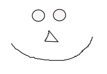
Computers, on the other hand, have a harder time looking at two circles and a few lines and saying, “Hey, this is a smiling face.”
Sensors and SDKs
The modern interest in computer vision as a consumer input for computer games has led to the development of several SDKs for performing computer-vision pattern recognition. One such system is Kinect for Windows. Although Microsoft provides a very high-level API with the Kinect, the downside is that you are locked into its hardware. The popular open source alternative is OpenCV, a library of computer-vision algorithms. Its advantage is that it can use a wide variety of camera hardware and not just the Kinect sensor.
Kinect
The Kinect was originally developed for the Xbox 360 but has recently been rebranded to include Kinect for Windows. As console game design has high entrance requirements, the Kinect for Windows allows more casual developers to try their hand at creating games with optical input. The system has a hardware component, called the Kinect sensor, and the previously mentioned Kinect SDK that does a lot of the heavy lifting for us in terms of pattern recognition and depth sensing. The hardware component consists of an infrared projector, infrared camera, visible light camera, and an array of microphones. The two cameras and the projector form the basis of the optical tracking system. The projector sends out infrared light that is invisible to humans. This light bounces off objects and is reflected back to the Kinect. The infrared camera records the reflected light pattern, and based on how it has been distorted, calculates how far the object is from the sensor. This exact method is carried out in the hardware of the sensor and is proprietary. However, the patent applications reveal that a special lens projects circles that, when reflected, become ellipses of varying shapes. The shape of the ellipse depends on the depth of the object reflecting it. In general, this is a much-improved version of depth from focus, in which the computer assumes that blurry objects are farther away than objects in focus.
As for object detection, the Kinect comes with a great set of algorithms for skeleton direction. It can also be trained to detect other objects, but skeleton detection is really its forte. The skeleton detection is good because of the massive amount of training Microsoft used for the algorithms when creating the SDK. If you were to use an average computer to run the Kinect skeleton training program, it would take about three years. Luckily, Microsoft had 1,000 computers lying around, so it takes them only a day to run the training simulation. This gives you an idea of the amount of training you need to provide for consumer-level tracking in your own algorithms. The Kinect can track up to six people with two of them being in “active” mode. For these 2 people, 20 individual joints are tracked. The sensor can also track people while standing or sitting.
OpenCV
The OpenCV method for 3D reconstruction is, well, more open! The library is designed to work with any common webcam or other camera you can get connected to your computer. OpenCV works well with stereoscopic cameras and is also capable of attempting to map depth with a single camera. However, those results would not be accurate enough to control a game, so we suggest you stick with two cameras if you’re trying to use regular webcams.
Indeed, finding depth is relatively straightforward using OpenCV. The built-in function
ReprojectImageTo3D calculates a vector for each pixel
(x,y) based on a disparity
map. A disparity map is a data set that describes how pixels have changed from one image to the
next; if you have stereoscopic cameras, this essentially is the reverse of the technique we
use in Chapter 24 when dealing with 3D displays. To create a disparity map,
OpenCV provides the handy function FindStereoCorrespondenceGC(). This function takes a set of images, assumes them
to be from a sterescopic source, and generates a disparity map by systematically comparing
them. The documentation is very complete, and there are several books on the subject of
OpenCV, including Learning OpenCV by Gary Bradski and Adrian Kaehler (O’Reilly), so we again will save the details for independent study.
Object detection is also possible with OpenCV. The common example in the OpenCV project uses Harr-like features to recognize objects. These features are rectangles whose mathematical structure allows for very fast computation. By developing patterns of these rectangles for a given object, a program can detect objects out of the background. For example, one such pattern could be if a selection rectangle includes an edge. The program would detect an edge in the pixel data by finding a sharp gradient between color and/or other attributes. If you detect the right number of edges in the right position, you have detected your object.
Hardcoding a pattern for the computer to look for would result in a very narrow set of recognition criteria. Therefore, computer-vision algorithms rely on a system of training rather than hard programming. Specifically, they use cascade classifier training.
The training process works well but requires a large image set. Typical examples require 6,000 negative images and 1,500 positive images. The negative images are commonly called background images. When training the algorithm, you take 1,200 of your positive images and draw selection rectangles around the object you are trying to detect. The computer learns that the pattern in the selection rectangles you’ve given it is one to be identified. This will take the average computer a long, long time. The remaining images are used for testing to ensure that your algorithm has satisfactory accuracy in detecting the patterns you’ve shown it. The larger the sample set, including different lighting, the more accurate the system will be. Once the algorithm is trained to detect a particular object, all you need is the training file—usually an .xml file—to share that training with another computer.
Numerical Differentiation
As previously noted, there are many ways to collect optical tracking data, but since we are focusing on the physics aspects, we’ll now talk about how to process the data to get meaningfully physical simulation. By combining object detection with depth sensing, we can detect and then track an object as it moves in the camera’s field of vision. Let’s assume that you have used the frame rate or internal clock to generate data of the following format:
{(x[i],y[i],z[i],t[i]),(x[i+1],y[i+1],z[i+1],t[i+1]) ,
(x[i+2],y[i+2],z[i+2],t[i+2]), ...}
Now, a single data point consisting of three coordinates and a timestamp doesn’t allow us to determine what is going on with an object’s velocity or acceleration. However, as the camera is supplying new position data at around 20–30 Hz, we will generate a time history of position or displacement. Using techniques similar to the numerical integration we used to take acceleration and turn it into velocities and then turn those velocities into position in earlier chapters, we can apply numerical differentiation to accomplish the reverse. Specifically, we can use the finite difference method.
For velocity, we need a first-order finite difference numerical differentiation scheme. Because we know the current data point and the previous data point, we are looking backward in time to get the current position. This is known as the backward difference scheme. In general, the backward difference is given by:
| f’(x) = lim h→0 (f(x+h) – f(x)) / h |
We must use the backward difference for the first-order differentiation, as we know only the present position and past positions. In our case, h is the difference in time between two data points and has a nonzero, fixed value. Therefore, the equation can be rewritten as:
| (f(x+h) – f(x)) / h = ∆f(x)/h |
where ∆f(x) is the position at the second timestamp minus the position at the first timestamp, and h is the difference in time. This is relatively straightforward, as we are just calculating the distance traveled divided by the time it took to travel that distance. This is the definition of average velocity.
Note that because we are finding the average velocity between the two data points, if the time delta, h, is too large, this will not accurately approximate the instantaneous velocity of the object. You may be tempted to push whatever hardware you have to its limit and get the highest possible sampling rate; however, if the time step is too small, the subtraction of one displacement from another will result in significant round-off error using floating-point arithmetic. You must take care to ensure that when you’re selecting a timestamp, (t[i] + h) – t[i] is exactly h. For more information on tuning these parameters, refer to the classic Numerical Recipes in C. The function to find velocity from our data structure would be as follows. Note that in our notation, t[i−1] is behind in time compared to t[i], so we are using the backward form. Your program needs to ensure that t[i−1] exists before executing this function:
Vector findVelocity (x[i-1], y[i-1], z[i-1], t[i-1], x[i], y[i], z[i], t[i]){

    float vx, vy, vz;

    vx = (x[i] − x[i-1])/(t[i]-t[i-1]);
    vy = (y[i] − y[i-1])/(t[i]-t[i-1]);
    vz = (z[i] − z[i-1])/(t[i]-t[i-1]);

    vector velocity = {vx, vy, vz};

    return velocity;

}
To compute the acceleration vector, we need to compare two velocities. However, we note that to get a velocity, we need two data points. Therefore, a total of three data points is required. The acceleration we solve for will actually be the acceleration for the middle data point as we compare the backward and forward difference. This technique is named the second-order central difference. In general, that form is as follows:
| f’’(x) = (f(x+2h) – 2f(x+h) + f(x)) / h2 |
This allows you to compute the acceleration directly without first finding the velocities. Here again, f(x) is the position reported by the sensor and h is the time step between data points. The same discussion of h applies here as well. Some tuning of the time step might be required to provide a stable differential. Of particular note with central difference forms is that periodic functions that are in sync with your time step may result in zero slope. If the motion you are tracking is periodic, you should take care to avoid a time step near the period of oscillation. This is called aliasing and is a problem with all signal analysis, including computer graphics displays. Also, note that this cannot be computed until at least three time steps have been stored. In our notation, t[i−1] is the center data point, t[i−2] the backward value, and t[i] the forward value. The acceleration function would therefore be as follows:
Vector findAcceleration (x[i-2], y[i-2], z[i-2], t[i-2], x[i-1], y[i-1], z[i-1],
                         t[i-1], x[i], y[i], z[i], t[i] ){

    float ax, ay, az, h;
    vector acceleration;

    h = t[i]-t[i-1];

    ax = (x[i] − 2*x[i-1] + x[i-2]) / h;
    ay = (y[i] − 2*y[i-1] + y[i-2]) / h;
    az = (z[i] − 2*z[i-1] + z[i-2]) / h;

    return acceleration = {ax, ay, az};
}
Now, let’s say that you are tracking a ball in someone’s hand. Until he lets it go, the velocity and acceleration we are calculating could change at any moment in any number of ways. It is not until the user lets go of the ball that the physics we have discussed takes over. Hence, you have to optically track it until he completes the throw. Once the ball is released, the physics from the rest of this book applies! You can then use the position at time of release, the velocity vector, and the acceleration vector to plot its trajectory in the game.