![]()
Vectors, Matrices, and Multidimensional Arrays
Vectors, matrices, and arrays of higher dimensions are essential tools in numerical computing. When a computation must be repeated for a set of input values, it is natural and advantageous to represent the data as arrays and the computation in terms of array operations. Computations that are formulated this way are said to be vectorized.1 Vectorized computing eliminates the need for many explicit loops over the array elements by applying batch operations on the array data. The result is concise and more maintainable code, and it enables delegating the implementation of (for example, elementwise) array operations to more efficient low-level libraries. Vectorized computations can therefore be significantly faster than sequential element-by-element computations. This is particularly important in an interpreted language such as Python, where looping over arrays element-by-element entails a significant performance overhead.
In Python's scientific computing environment, efficient data structures for working with arrays are provided by the NumPy library. The core of NumPy is implemented in C, and provide efficient functions for manipulating and processing arrays. At a first glance, NumPy arrays bear some resemblance to Python’s list data structure. But an important difference is that while Python lists are generic containers of objects, NumPy arrays are homogenous and typed arrays of fixed size. Homogenous means that all elements in the array have the same data type. Fixed size means that an array cannot be resized (without creating a new array). For these and other reasons, operations and functions acting on NumPy arrays can be much more efficient than operations on Python lists. In addition to the data structures for arrays, NumPy also provides a large collection of basic operators and functions that act on these data structures, as well as submodules with higher-level algorithms such as linear algebra and fast Fourier transformations.
In this chapter we first look at the basic NumPy data structure for arrays and various methods to create such NumPy arrays. Next we look at operations for manipulating arrays and for doing computations with arrays. The multidimensional data array provided by NumPy is a foundation for nearly all numerical libraries for Python. Spending time on getting familiar with NumPy and develop an understanding for how NumPy works is therefore important.
![]() NumPy The NumPy library provides data structures for representing a rich variety of arrays, and methods and functions for operating on such arrays. NumPy provides the numerical back end for nearly every scientific or technical library for Python. It is therefore a very important part of the scientific Python ecosystem. At the time of writing, the latest version of NumPy is 1.9.2. More information about NumPy is available at http://www.numpy.org.
NumPy The NumPy library provides data structures for representing a rich variety of arrays, and methods and functions for operating on such arrays. NumPy provides the numerical back end for nearly every scientific or technical library for Python. It is therefore a very important part of the scientific Python ecosystem. At the time of writing, the latest version of NumPy is 1.9.2. More information about NumPy is available at http://www.numpy.org.
Importing NumPy
In order to use the NumPy library, we need to import it in our program. By convention, the numpy module imported under the alias np, like so:
In [1]: import numpy as np
After this, we can access functions and classes in the numpy module using the np namespace. Throughout this book, we assume that the NumPy module is imported in this way.
The NumPy Array Object
The core of the NumPy library is the data structures for representing multidimensional arrays of homogeneous data. Homogeneous refers to that all elements in an array have the same data type.2 The main data structure for multidimensional arrays in NumPy is the ndarray class. In addition to the data stored in the array, this data structure also contains important metadata about the array, such as its shape, size, data type, and other attributes. See Table 2-1 for a more detailed description of these attributes. A full list of attributes with descriptions is available in the ndarray docstring, which can be accessed by calling help(np.ndarray) in the Python interpreter or np.ndarray? in an IPython console.
Table 2-1. Basic attributes of the ndarray class
|
Attribute |
Description |
|---|---|
|
shape |
A tuple that contains the number of elements (i.e., the length) for each dimension (axis) of the array. |
|
size |
The total number of elements in the array. |
|
ndim |
Number of dimensions (axes). |
|
nbytes |
Number of bytes used to store the data. |
|
dtype |
The data type of the elements in the array. |
The following example demonstrates how these attributes are accessed for an instance data of the class ndarray:
In [2]: data = np.array([[1, 2], [3, 4], [5, 6]])
In [3]: type(data)
Out[3]: <class 'numpy.ndarray'>
In [4]: data
Out[4]: array([[1, 2],
               [3, 4],
               [5, 6]])
In [5]: data.ndim
Out[5]: 2
In [6]: data.shape
Out[6]: (3, 2)
In [7]: data.size
Out[7]: 6
In [8]: data.dtype
Out[8]: dtype('int64')
In [9]: data.nbytes
Out[9]: 48
Here the ndarray instance data is created from a nested Python list using the function np.array. The following section introduces more ways to create ndarray instances from data and from rules of various kinds. In the example above, the data is a two-dimensional array (data.ndim) of shape ![]() , as indicated by data.shape, and in total it contains 6 elements (data.size) of type int64 (data.dtype), which amounts to a total size of 48 bytes (data.nbytes).
, as indicated by data.shape, and in total it contains 6 elements (data.size) of type int64 (data.dtype), which amounts to a total size of 48 bytes (data.nbytes).
In the previous section we encountered the dtype attribute of the ndarray object. This attribute describes the data type of each element in the array (remember, since NumPy arrays are homogeneous, all elements have the same data type). The basic numerical data types supported in NumPy are shown in Table 2-2. Non-numerical data types, such as strings, objects, and user-defined compound types are also supported.
Table 2-2. Basic numerical data types available in NumPy
|
dtype |
Variants |
Description |
|---|---|---|
|
int |
int8, int16, int32, int64 |
Integers. |
|
uint |
uint8, uint16, uint32, uint64 |
Unsigned (non-negative) integers. |
|
bool |
bool |
Boolean (True or False). |
|
float |
float16, float32, float64, float128 |
Floating-point numbers. |
|
complex |
complex64, complex128, complex256 |
Complex-valued floating-point numbers. |
For numerical work the most important data types are int (for integers), float (for floating-point numbers) and complex (complex floating-point numbers). Each of these data types come in different sizes, such as int32 for 32-bit integers, int64 for 64-bit integers, etc. This offers more fine-grained control over data types than the standard Python types, which only provides one type for integers and one type for floats. It is usually not necessary to explicitly choose the bit size of the data type to work with, but it is often necessary to explicitly choose whether to use arrays of integers, floating-point numbers, or complex values.
The following example demonstrates how to use the dtype attribute to generate arrays of integer-, float-, and complex-valued elements:
In [10]: np.array([1, 2, 3], dtype=np.int)
Out[10]: array([1, 2, 3])
In [11]: np.array([1, 2, 3], dtype=np.float)
Out[11]: array([ 1.,  2.,  3.])
In [12]: np.array([1, 2, 3], dtype=np.complex)
Out[12]: array([ 1.+0.j,  2.+0.j,  3.+0.j])
Once a NumPy array is created its dtype cannot be changed, other than by creating a new copy with type-casted array values. Typecasting an array is straightforward, and can be done using either the np.array function:
In [13]: data = np.array([1, 2, 3], dtype=np.float)
In [14]: data
Out[14]: array([ 1.,  2.,  3.])
In [15]: data.dtype
Out[15]: dtype('float64')
In [16]: data = np.array(data, dtype=np.int)
In [17]: data.dtype
Out[17]: dtype('int64')
In [18]: data
Out[18]: array([1, 2, 3])
or by using the astype attribute of the ndarray class:
In [19]: data = np.array([1, 2, 3], dtype=np.float)
In [20]: data
Out[20]: array([ 1.,  2.,  3.])
In [21]: data.astype(np.int)
Out[21]: array([1, 2, 3])
When computing with NumPy arrays, the data type might get promoted from one type to another, if required by the operation. For example, adding float-valued and complex-valued arrays, the resulting array is a complex-valued array:
In [22]: d1 = np.array([1, 2, 3], dtype=float)
In [23]: d2 = np.array([1, 2, 3], dtype=complex)
In [24]: d1 + d2
Out[24]: array([ 2.+0.j,  4.+0.j,  6.+0.j])
In [25]: (d1 + d2).dtype
Out[25]: dtype('complex128')
In some cases, depending on the application and its requirements, it is essential to create arrays with data type appropriately set to, for example, int or complex. The default type is float. Consider the following example:
In [26]: np.sqrt(np.array([-1, 0, 1]))
Out[26]: RuntimeWarning: invalid value encountered in sqrt
         array([ nan,   0.,   1.])
In [27]: np.sqrt(np.array([-1, 0, 1], dtype=complex))
Out[27]: array([ 0.+1.j,  0.+0.j,  1.+0.j])
Here, using the np.sqrt function to compute the square root of each element in an array gives different results depending on the data type of the array. Only when the data type of the array is complex is the square root of -1 giving in the imaginary unit (denoted as 1j in Python).
Regardless of the value of the dtype attribute, all NumPy array instances have the attributes real and imag for extracting the real and imaginary parts of the array, respectively:
In [28]: data = np.array([1, 2, 3], dtype=complex)
In [29]: data
Out[29]: array([ 1.+0.j,  2.+0.j,  3.+0.j])
In [30]: data.real
Out[30]: array([ 1.,  2.,  3.])
In [31]: data.imag
Out[31]: array([ 0.,  0.,  0.])
The same functionality is also provided by the functions np.real and np.imag, which also can be applied to other array-like objects, such as Python lists. Note that Python itself has support of complex numbers, and the imag and real attributes are also available for Python scalars.
Order of Array Data in Memory
Multidimensional arrays are stored as contiguous data in memory. There is a freedom of choice in how to arrange the array elements in this memory segment. Consider the case of a two-dimensional array, containing rows and columns: One possible way to store this array as a consecutive sequence of values is to store the rows after each other, and another equally valid approach is to store the columns one after another. The former is called row-major format and the latter is column-major format. Whether to use row-major or column-major is a matter of conventions, and row-major format is used for example in the C programming language, and Fortran uses the column-major format. A NumPy array can be specified to be stored in row-major format, using the keyword argument order='C', and column-major format, using the keyword argument order='F', when the array is created or reshaped. The default format is row-major. The 'C' or 'F' ordering of NumPy array is particularly relevant when NumPy arrays are used in interfacing software written in C and Fortran, which is frequently required when working with numerical computing with Python.
Row-major and column-major ordering are special cases of strategies for mapping the index used to address an element, to the offset for the element in the array’s memory segment. In general, the NumPy array attribute ndarray.strides defines exactly how this mapping is done. The strides attribute is a tuple of the same length as the number of axes (dimensions) of the array. Each value in strides is the factor by which the index for the corresponding axis is multiplied when calculating the memory offset (in bytes) for a given index expression.
For example, consider a C-order array A with shape (2, 3), which corresponds to a two-dimensional array with two and three elements along the first and the second dimension, respectively. If the data type is int32, then each element uses 4 bytes, and the total memory buffer for the array therefore uses ![]() bytes. The strides attribute of this array is therefore
bytes. The strides attribute of this array is therefore ![]() , because each increment of m in A[n, m] increases the memory offset with 1 item, or 4 bytes. Likewise, each increment of n increases the memory offset with 3 items, or 12 bytes (because the second dimension of the array has length 3). If, on the other hand, the same array were stored in 'F' order, the strides would instead be (4, 8). Using strides to describe the mapping of array index to array memory offset is clever because it can be used to describe different mapping strategies, and many common operations on arrays, such as for example the transpose, can be implemented by simply changing the strides attribute, which can eliminate the need for moving data around in the memory. Operations that only require changing the strides attribute result in new ndarray objects that refer to the same data as the original array. Such arrays are called views. For efficiency, NumPy strives to create views rather than copies of arrays when applying operations on arrays. This is generally a good thing, but it is important to be aware of that some array operations results in views rather than new independent arrays, because modifying their data also modifies the data of the original array. Later in this chapter we will see several examples of this behavior.
, because each increment of m in A[n, m] increases the memory offset with 1 item, or 4 bytes. Likewise, each increment of n increases the memory offset with 3 items, or 12 bytes (because the second dimension of the array has length 3). If, on the other hand, the same array were stored in 'F' order, the strides would instead be (4, 8). Using strides to describe the mapping of array index to array memory offset is clever because it can be used to describe different mapping strategies, and many common operations on arrays, such as for example the transpose, can be implemented by simply changing the strides attribute, which can eliminate the need for moving data around in the memory. Operations that only require changing the strides attribute result in new ndarray objects that refer to the same data as the original array. Such arrays are called views. For efficiency, NumPy strives to create views rather than copies of arrays when applying operations on arrays. This is generally a good thing, but it is important to be aware of that some array operations results in views rather than new independent arrays, because modifying their data also modifies the data of the original array. Later in this chapter we will see several examples of this behavior.
Creating Arrays
In the previous section, we looked at NumPy's basic data structure for representing arrays, the ndarray class, and we looked at basic attributes of this class. In this section we focus on functions from the NumPy library that can be used to create ndarray instances.
Arrays can be generated in a number of ways, depending their properties and the applications they are used for. For example, as we saw in the previous section, one way to initialize an ndarray instance is to use the np.array function on a Python list, which, for example, can be explicitly defined. However, this method is obviously limited to small arrays. In many situations it is necessary to generate arrays with elements that follow some given rule, such as filled with constant values, increasing integers, uniformly spaced numbers, random numbers, etc. In other cases we might need to create arrays from data stored in a file. The requirements are many and varied, and the NumPy library provides a comprehensive set of functions for generating arrays of various types. In this section we look in more detail at many of these functions. For a complete list, see the NumPy reference manual or the docstrings that is available by typing help(np) or using the autocompletion np.<TAB>. A summary of frequently used array-generating functions is given in Table 2-3.
Table 2-3. Summary of NumPy functions for generating arrays
|
Function name |
Type of array |
|---|---|
|
np.array |
Creates an array for which the elements are given by an array-like object, which, for example, can be a (nested) Python list, a tuple, an iterable sequence, or another ndarray instance. |
|
np.zeros |
Creates an array – with the specified dimensions and data type – that is filled with zeros. |
|
np.ones |
Creates an array – with the specified dimensions and data type – that is filled with ones. |
|
np.diag |
Creates a diagonal array with specified values along the diagonal, and zeros elsewhere. |
|
np.arange |
Creates an array with evenly spaced values between specified start, end, and increment values. |
|
np.linspace |
Creates an array with evenly spaced values between specified start and end values, using a specified number of elements. |
|
np.logspace |
Creates an array with values that are logarithmically spaced between the given start and end values. |
|
np.meshgrid |
Generate coordinate matrices (and higher-dimensional coordinate arrays) from one-dimensional coordinate vectors. |
|
np.fromfunction |
Create an array and fill it with values specified by a given function, which is evaluated for each combination of indices for the given array size. |
|
np.fromfile |
Create an array with the data from a binary (or text) file. NumPy also provides a corresponding function np.tofile with which NumPy arrays can be stored to disk, and later read back using np.fromfile. |
|
np.genfromtxt, np.loadtxt |
Creates an array from data read from a text file. For example, a comma-separated value (CSV) file. The function np.genfromtxt also supports data files with missing values. |
|
np.random.rand |
Generates an array with random numbers that are uniformly distributed between 0 and 1. Other types of distributions are also available in the np.random module. |
Arrays Created from Lists and Other Array-like Objects
Using the np.array function, NumPy arrays can be constructed from explicit Python lists, iterable expressions, and other array-like objects (such as other ndarray instances). For example, to create a one-dimensional array from a Python list, we simply pass the Python list as an argument to the np.array function:
In [32]: np.array([1, 2, 3, 4])
Out[32]: array([ 1,  2,  3, 4])
In [33]: data.ndim
Out[33]: 1
In [34]: data.shape
Out[34]: (4,)
To create a two-dimensional array with the same data as in the previous example, we can use a nested Python list:
In [35]: np.array([[1, 2], [3, 4]])
Out[35]: array([[1, 2],
                [3, 4]])
In [36]: data.ndim
Out[36]: 2
In [37]: data.shape
Out[37]: (2, 2)
Arrays Filled with Constant Values
The functions np.zeros and np.ones create and return arrays filled with zeros and ones, respectively. They take, as first argument, an integer or a tuple that describes the number of elements along each dimension of the array. For example, to create a ![]() array filled with zeros, and an array of length 4 filled with ones, we can use:
array filled with zeros, and an array of length 4 filled with ones, we can use:
In [38]: np.zeros((2, 3))
Out[38]: array([[ 0.,  0.,  0.],
                [ 0.,  0.,  0.]])
In [39]: np.ones(4)
Out[39]: array([ 1.,  1.,  1., 1.])
Like other array-generating functions, the np.zeros and np.ones functions also accept an optional keyword argument that specifies the data type for the elements in the array. By default, the data type is float64, and it can be changed to the required type by explicitly specify the dtype argument.
In [40]: data = np.ones(4)
In [41]: data.dtype
Out[41]: dtype('float64')
In [42]: data = np.ones(4, dtype=np.int64)
In [43]: data.dtype
Out[43]: dtype('int64')
An array filled with an arbitrary constant value can be generated by first creating an array filled with ones, and then multiply the array with the desired fill value. However, NumPy also provides the function np.full that does exactly this in one step. The following two ways of constructing arrays with 10 elements, which are initialized to the numerical value 5.4 in this example, produces the same results, but using np.full is slightly more efficient since it avoids the multiplication.
In [44]: x1 = 5.4 * np.ones(10)
In [45]: x2 = np.full(10, 5.4)
An already created array can also be filled with constant values using the np.fill function, which takes an array and a value as arguments, and set all elements in the array to the given value. The following two methods to create an array therefore give the same results:
In [46]: x1 = np.empty(5)
In [47]: x1.fill(3.0)
In [48]: x1
Out[48]: array([ 3.,  3.,  3.,  3.,  3.])
In [49]: x2 = np.full(5, 3.0)
In [50]: x2
Out[50]: array([ 3.,  3.,  3.,  3.,  3.])
In this last example we also used the np.empty function, which generates an array with uninitialized values, of the given size. This function should only be used when the initialization of all elements can be guaranteed by other means, such as an explicit loop over the array elements or another explicit assignment. This function is described in more detail later in this chapter.
Arrays Filled with Incremental Sequences
In numerical computing it is very common to require arrays with evenly spaced values between a start value and end value. NumPy provides two similar functions to create such arrays: np.arange and np.linspace. Both functions takes three arguments, where the first two arguments are the start and end values. The third argument of np.arange is the increment, while for np.linspace it is the total number of points in the array.
For example, to generate arrays with values between 1 and 10, with increment 1, we could use either of the following:
In [51]: np.arange(0.0, 10, 1)
Out[51]: array([ 0.,  1.,  2.,  3.,  4.,  5.,  6.,  7.,  8.,  9.])
In [52]: np.linspace(0, 10, 11)
Out[52]: array([ 0.,  1.,  2.,  3.,  4.,  5.,  6.,  7.,  8.,  9.,  10.])
However, note that np.arange does not include the end value (10), while by default np.linspace does (although this behavior can be changed using the optional endpoint keyword argument). Whether to use np.arange or np.linspace is mostly a matter of personal preference, but it is generally recommended to use np.linspace whenever the increment is a non-integer.
Arrays Filled with Logarithmic Sequences
The function np.logspace is similar to np.linspace, but the increments between the elements in the array are logarithmically distributed, and the first two arguments are the powers of the optional base keyword argument (which defaults to 10) for the start and end values. For example, to generate an array with logarithmically distributed values between 1 and 100, we can use:
In [53]: np.logspace(0, 2, 5)  # 5 data points between 10**0=1 to 10**2=100
Out[53]: array([ 1. , 3.16227766, 10. , 31.6227766 , 100.])
Multidimensional coordinate grids can be generated using the function np.meshgrid. Given two one-dimensional coordinate arrays (that is, arrays containing a set of coordinates along a given dimension), we can generate two-dimensional coordinate arrays using the np.meshgrid function. An illustration of this is given in the following example:
In [54]: x = np.array([-1, 0, 1])
In [55]: y = np.array([-2, 0, 2])
In [56]: X, Y = np.meshgrid(x, y)
In [57]: X
Out[57]: array([[-1,  0,  1],
                [-1,  0,  1],
                [-1,  0,  1]])
In [58]: Y
Out[58]: array([[-2, -2, -2],
                [ 0,  0,  0],
                [ 2,  2,  2]])
A common use-case of the two-dimensional coordinate arrays, like X and Y in this example, is to evaluate functions over two variables x and y. This can be used when plotting functions over two variables, as color-map plots and contour plots. For example, to evaluate the expression ![]() at all combinations of values from the x and y arrays above, we can use the two-dimensional coordinate arrays X and Y:
at all combinations of values from the x and y arrays above, we can use the two-dimensional coordinate arrays X and Y:
In [59]: Z = (X + Y) ** 2
In [60]: Z
Out[60]: array([[9, 4, 1],
                [1, 0, 1],
                [1, 4, 9]])
It is also possible to generate higher-dimensional coordinate arrays by passing more arrays as argument to the np.meshgrid function. Alternatively, the functions np.mgrid and np.ogrid can also be used to generate coordinate arrays, using a slightly different syntax based on indexing and slice objects. See their docstrings or the NumPy documentation for details.
Creating Uninitialized Arrays
To create an array of specific size and data type, but without initializing the elements in the array to any particular values, we can use the function np.empty. The advantage of using this function, for example, instead of np.zeros, which creates an array initialized with zero-valued elements, is that we can avoid the initiation step. If all elements are guaranteed to be initialized later in the code, this can save a little bit of time, especially when working with large arrays. To illustrate the use of the np.empty function, consider the following example:
In [61]: np.empty(3, dtype=np.float)
Out[61]: array([  1.28822975e-231,   1.28822975e-231,   2.13677905e-314])
Here we generated a new array with three elements of type float. There is no guarantee that the elements have any particular values, and the actual values will vary from time to time. For this reason is it important that all values are explicitly assigned before the array is used, otherwise unpredictable errors are likely to arise. Often the np.zeros function is a safer alternative to np.empty, and if the performance gain is not essential it is better to use np.zeros, to minimize the likelihood of subtle and hard to reproduce bugs due to uninitialized values in the array returned by np.empty.
Creating Arrays with Properties of Other Arrays
It is often necessary to create new arrays that share properties, such as shape and data type, with another array. NumPy provides a family of functions for this purpose: np.ones_like, np.zeros_like, np.full_like, and np.empty_like. A typical use-case is a function that takes arrays of unspecified type and size as arguments, and requires working arrays of the same size and type. For example, a boilerplate example of this situation is given in the following function:
def f(x):
    y = np.ones_like(x)
    # compute with x and y
    return y
At the first line of the body of this function, a new array y is created using np.ones_like, which results in an array of the same size and data type as x, and filled with ones.
Creating Matrix Arrays
Matrices, or two-dimensional arrays, are an important case for numerical computing. NumPy provides functions for generating commonly used matrices. In particular, the function np.identity generates a square matrix with ones on the diagonal and zeros elsewhere:
In [62]: np.identity(4)
Out[62]: array([[ 1.,  0.,  0.,  0.],
                [ 0.,  1.,  0.,  0.],
                [ 0.,  0.,  1.,  0.],
                [ 0.,  0.,  0.,  1.]])
The similar function numpy.eye generates matrices with ones on a diagonal (optionally offset), as illustrated in the following example, which produces matrices with nonzero diagonals above and below the diagonal, respectively:
In [63]: np.eye(3, k=1)
Out[63]: array([[ 0.,  1.,  0.],
                [ 0.,  0.,  1.],
                [ 0.,  0.,  0.]])
In [64]: np.eye(3, k=-1)
Out[64]: array([[ 0.,  0.,  0.],
                [ 1.,  0.,  0.],
                [ 0.,  1.,  0.]])
To construct a matrix with an arbitrary one-dimensional array on the diagonal we can use the np.diag function (which also takes the optional keyword argument k to specify an offset from the diagonal), as demonstrated here:
In [65]: np.diag(np.arange(0, 20, 5))
Out[65]: array([[0,  0,  0,  0],
                [0,  5,  0,  0],
                [0,  0, 10,  0],
                [0,  0,  0, 15]])
Here we gave a third argument to the np.arange function, which specifies the step size in the enumeration of elements in the array returned by the function. The resulting array therefore contains the values [0, 5, 10, 15], which are inserted on the diagonal of a two-dimensional matrix by the np.diag function.
Indexing and Slicing
Elements and subarrays of NumPy arrays are accessed using the standard square bracket notation that is also used with for example Python lists. Within the square bracket, a variety of different index formats are used for different types of element selection. In general, the expression within the bracket is a tuple, where each item in the tuple is a specification of which elements to select from each axis (dimension) of the array.
One-dimensional Arrays
Along a single axis, integers are used to select single elements, and so-called slices are used to select ranges and sequences of elements. Positive integers are used to index elements from the beginning of the array (index starts at 0), and negative integers are used to index elements from the end of the array, where the last element is indexed with -1, the second-to-last element with -2, and so on.
Slices are specified using the : notation that is also used for Python lists. In this notation, a range of elements can be selected using an expressions like m:n, which selects elements starting with m and ending with ![]() (note that the nth element is not included). The slice m:n can also be written more explicitly as m:n:1, where the number 1 specifies that every element between m and n should be selected. To select every second element between m and n, use m:n:2, and to select every p element, use m:n:p, and so on. If p is negative, elements are returned in reversed order starting from m to
(note that the nth element is not included). The slice m:n can also be written more explicitly as m:n:1, where the number 1 specifies that every element between m and n should be selected. To select every second element between m and n, use m:n:2, and to select every p element, use m:n:p, and so on. If p is negative, elements are returned in reversed order starting from m to ![]() (which implies that m has be larger than n in this case). See Table 2-4 for a summary of indexing and slicing operations for NumPy arrays.
(which implies that m has be larger than n in this case). See Table 2-4 for a summary of indexing and slicing operations for NumPy arrays.
Table 2-4. Examples of array indexing and slicing expressions
|
Expression |
Description |
|---|---|
|
a[m] |
Select element at index m, where m is an integer (start counting form 0). |
|
a[-m] |
Select the mth element from the end of the list, where m is an integer. The last element in the list is addressed as -1, the second-to-last element as -2, and so on. |
|
a[m:n] |
Select elements with index starting at m and ending at |
|
a[:] or a[0:-1] |
Select all elements in the given axis. |
|
a[:n] |
Select elements starting with index 0 and going up to index |
|
a[m:] or a[m:-1] |
Select elements starting with index m (integer) and going up to the last element in the array. |
|
a[m:n:p] |
Select elements with index m through n (exclusive), with increment p. |
|
a[::-1] |
Select all the elements, in reverse order. |
The following examples demonstrate index and slicing operations for NumPy arrays. To begin with, consider an array with a single axis (dimension) that contains a sequence of integers between 0 and 10:
In [66]: a = np.arange(0, 11)
In [67]: a
Out[67]: array([ 0,  1,  2,  3,  4,  5,  6,  7,  8,  9, 10])
Note that the end value 11 is not included in the array. To select specific elements from this array, for example the first, the last, and the 5th element we can use integer indexing:
In [68]: a[0]  # the first element
Out[68]: 0
In [69]: a[-1] # the last element
Out[69]: 10
In [70]: a[4]  # the fifth element, at index 4
Out[70]: 4
To select a range of elements, say from the second to the second-to-last element, selecting every element and every second element, respectively, we can use index slices:
In [71]: a[1:-1]
Out[71]: array([1, 2, 3, 4, 5, 6, 7, 8, 9])
In [72]: a[1:-1:2]
Out[72]: array([1, 3, 5, 7, 9])
To select the first five and the last five elements from an array, we can use the slices :5 and -5:, since if m or n is omitted in m:n, the defaults are the beginning and the end of the array, respectively.
In [73]: a[:5]
Out[73]: array([0, 1, 2, 3, 4])
In [74]: a[-5:]
Out[74]: array([6, 7, 8, 9, 10])
To reverse the array and select only every second value, we can use the slice ::-2, as shown in the following example:
In [75]: a[::-2]
Out[75]: array([10,  8,  6,  4,  2,  0])
Multidimensional Arrays
With multidimensional arrays, element selections like those introduced in the previous section can be applied on each axis (dimension). The result is a reduced array where each element matches the given selection rules. As a specific example, consider the following two-dimensional array:
In [76]: f = lambda m, n: n + 10 * m
In [77]: A = np.fromfunction(f, (6, 6), dtype=int)
In [78]: A
Out[78]: array([[ 0,  1,  2,  3,  4,  5],
                [10, 11, 12, 13, 14, 15],
                [20, 21, 22, 23, 24, 25],
                [30, 31, 32, 33, 34, 35],
                [40, 41, 42, 43, 44, 45],
                [50, 51, 52, 53, 54, 55]])
We can extract columns and rows from this two-dimensional array using a combination of slice and integer indexing:
In [79]: A[:, 1]  # the second column
Out[79]: array([ 1, 11, 21, 31, 41, 51])
In [80]: A[1, :]  # the second row
Out[80]: array([10, 11, 12, 13, 14, 15])
By applying a slice on each of the array axes, we can extract subarrays (submatrices in this two-dimensional example):
In [81]: A[:3, :3]  # upper half diagonal block matrix
Out[81]: array([[ 0,  1,  2],
                [10, 11, 12],
                [20, 21, 22]])
In [82]: A[3:, :3]  # lower left off-diagonal block matrix
Out[82]: array([[30, 31, 32],
                [40, 41, 42],
                [50, 51, 52]])
With element spacing other that 1, submatrices made up from nonconsecutive elements can be extracted:
In [83]: A[::2, ::2]  # every second element starting from 0, 0
Out[83]: array([[ 0,  2,  4],
                [20, 22, 24],
                [40, 42, 44]])
In [84]: A[1::2, 1::3]  # every second and third element starting from 1, 1
Out[84]: array([[11, 14],
                [31, 34],
                [51, 54]])
This ability to extract subsets of data from a multidimensional array is a simple but very powerful feature that is useful in many data processing applications.
Views
Subarrays that are extracted from arrays using slice operations are alternative views of the same underlying array data. That is, they are arrays that refer to the same data in memory as the original array, but with a different strides configuration. When elements in a view are assigned new values, the values of the original array are therefore also updated. For example,
In [85]: B = A[1:5, 1:5]
In [86]: B
Out[86]: array([[11, 12, 13, 14],
                [21, 22, 23, 24],
                [31, 32, 33, 34],
                [41, 42, 43, 44]])
In [87]: B[:, :] = 0
In [88]: A
Out[88]: array([[ 0,  1,  2,  3,  4,  5],
                [10,  0,  0,  0,  0, 15],
                [20,  0,  0,  0,  0, 25],
                [30,  0,  0,  0,  0, 35],
                [40,  0,  0,  0,  0, 45],
                [50, 51, 52, 53, 54, 55]])
Here, assigning new values to the elements in an array B, which is created from the array A, also modifies the values in A (since both arrays refer to the same data in the memory). The fact that extracting subarrays results in views rather than new independent arrays eliminates the need for copying data and improves performance. When a copy rather than a view is needed, the view can be copied explicitly by using the copy method of the ndarray instance.
In [89]: C = B[1:3, 1:3].copy()
In [90]: C
Out[90]: array([[0, 0],
                [0, 0]])
In [91]: C[:, :] = 1  # this does not affect B since C is a copy of the view B[1:3, 1:3]
In [92]: C
Out[92]: array([[1, 1],
                [1, 1]])
In [93]: B
Out[93]: array([[0, 0, 0, 0],
                [0, 0, 0, 0],
                [0, 0, 0, 0],
                [0, 0, 0, 0]])
In addition to the copy attribute of the ndarray class, an array can also be copied using the function np.copy, or, equivalently, using the np.array function with the keyword argument copy=True.
Fancy Indexing and Boolean-valued Indexing
In the previous section we looked at indexing NumPy arrays with integers and slices, to extract individual elements or ranges of elements. NumPy provides another convenient method to index arrays, called fancy indexing. With fancy indexing, an array can be indexed with another NumPy array, a Python list, or a sequence of integers, whose values select elements in the indexed array. To clarify this concept, consider the following example: we first create a NumPy array with 11 floating-point numbers, and then index the array with another NumPy array (or Python list), to extract element number 0, 2 and 4 from the original array:
In [94]: A = np.linspace(0, 1, 11)
Out[94]: array([ 0. ,  0.1,  0.2,  0.3,  0.4,  0.5,  0.6,  0.7,  0.8,  0.9,  1. ])
In [95]: A[np.array([0, 2, 4])]
Out[95]: array([ 0. ,  0.2,  0.4])
In [96]: A[[0, 2, 4]]  # The same thing can be accomplished by indexing with a Python list
Out[96]: array([ 0. ,  0.2,  0.4])
This method of indexing can be used along each axis (dimension) of a multidimensional NumPy array. It requires that the elements in the array or list used for indexing are integers.
Another variant of indexing NumPy arrays with another NumPy array uses Boolean-valued index arrays. In this case, each element (with values True or False) indicates whether or not to select the element from the array with the corresponding index. That is, if element n in the indexing array of Boolean values is True, then element n is selected from the indexed array. If the value is False, then element n is not selected. This index method is handy when filtering out elements from an array. For example, to select all the elements from the array A (as defined above) that exceed the value 0.5, we can use the following combination of the comparison operator applied to a NumPy array, and array indexing using a Boolean-valued array:
In [97]: A > 0.5
Out[97]: array([False, False, False, False, False, False, True, True, True, True, True],
         dtype=bool)
In [98]: A[A > 0.5]
Out[98]: array([ 0.6,  0.7,  0.8,  0.9,  1. ])
Unlike arrays created by using slices, the arrays returned using fancy indexing and Boolean-valued indexing are not views, but rather new independent arrays. Nonetheless, it is possible to assign values to elements selected using fancy indexing:
In [99]: A = np.arange(10)
In [100]: indices = [2, 4, 6]
In [101]: B = A[indices]
In [102]: B[0] = -1  # this does not affect A
In [103]: A
Out[103]: array([0, 1, 2, 3, 4, 5, 6, 7, 8, 9])
In [104]: A[indices] = -1
In [105]: A
Out[105]: array([ 0,  1, -1,  3, -1,  5, -1,  7,  8,  9])
and likewise for Boolean-valued indexing:
In [106]: A = np.arange(10)
In [107]: B = A[A > 5]
In [108]: B[0] = -1  # this does not affect A
In [109]: A
Out[109]: array([0, 1, 2, 3, 4, 5, 6, 7, 8, 9])
In [110]: A[A > 5] = -1
In [111]: A
Out[111]: array([ 0,  1,  2,  3,  4,  5, -1, -1, -1, -1])
A visual summary of different methods to index NumPy arrays is given in Figure 2-1. Note that each type of indexing we have discussed here can be independently applied to each dimension of an array.
Reshaping and Resizing
When working with data in array form, it is often useful to rearrange arrays and alter the way they are interpreted. For example, an ![]() matrix array could be rearranged into a vector of length N2, or a set of one-dimensional arrays could be concatenated together, or stacked next to each other to form a matrix. NumPy provides a rich set of functions of this type of manipulation. See the Table 2-5 for a summary of a selection of these functions.
matrix array could be rearranged into a vector of length N2, or a set of one-dimensional arrays could be concatenated together, or stacked next to each other to form a matrix. NumPy provides a rich set of functions of this type of manipulation. See the Table 2-5 for a summary of a selection of these functions.

Figure 2-1. Visual summary of indexing methods for NumPy arrays. These diagrams represent NumPy arrays of shape (4, 4), and the highlighted elements are those that are selected using the indexing expression shown above the block representations of the arrays
Table 2-5. Summary of NumPy functions for manipulating the dimensions and the shape of arrays
|
Function / method |
Description |
|---|---|
|
np.reshape, np.ndarray.reshape |
Reshape an N-dimensional array. The total number of elements must remain the same. |
|
np.ndarray.flatten |
Create a copy of an N-dimensional array and reinterpret it as a one-dimensional array (that is, all dimensions are collapsed into one). |
|
np.ravel, np.ndarray.ravel |
Create a view (if possible, otherwise a copy) of an N-dimensional array in which it is interpreted as a one-dimensional array. |
|
np.squeeze |
Remove axes with length 1. |
|
np.expand_dims, np.newaxis |
Adds a new axis (dimension) of length 1 to an array, where np.newaxis is used with array indexing. |
|
np.transpose, np.ndarray.transpose, np.ndarray.T |
Transpose the array. The transpose operation corresponds to reversing (or more generally, permuting) the axes of the array. |
|
np.hstack |
Stack a list of arrays horizontally (along axis 1): For example, given a list of column vectors, append the columns to form a matrix. |
|
np.vstack |
Stack a list of arrays vertically (along axis 0): For example, given a list of row vectors, append the rows to form a matrix. |
|
np.dstack |
Stack arrays depth-wise (along axis 2). |
|
np.concatenate |
Create a new array by appending arrays after each other, along a given axis. |
|
np.resize |
Resize an array. Creates a new copy of the original array, with the requested size. If necessary, the orignal array will repeated to fill up the new array. |
|
np.append |
Append an element to an array. Creates a new copy of the array. |
|
np.insert |
Insert a new element at a given position. Creates a new copy of the array. |
|
np.delete |
Delete an element at a given position. Creates a new copy of the array. |
Reshaping an array does not require modifying the underlying array data; it only changes in how the data is interpreted, by redefining the array’s strides attribute. An example of this type of operation is a ![]() array (matrix) that is reinterpreted as a
array (matrix) that is reinterpreted as a ![]() array (vector). In NumPy, the function np.reshape, or the ndarray class method reshape, can be used to reconfigure how the underlying data is interpreted. It takes an array and the new shape of the array as arguments:
array (vector). In NumPy, the function np.reshape, or the ndarray class method reshape, can be used to reconfigure how the underlying data is interpreted. It takes an array and the new shape of the array as arguments:
In [112]: data = np.array([[1, 2], [3, 4]])
In [113]: np.reshape(data, (1, 4))
Out[113]: array([[1, 2, 3, 4]])
In [114]: data.reshape(4)
Out[114]: array([1, 2, 3, 4])
It is necessary that the requested new shape of the array match the number of elements in the original size. However, the number axes (dimensions) does not need to be conserved, as illustrated in the previous example, where in the first case the new array has dimension 2 and shape (1,4), while in the second case the new array has dimension 1 and shape (4,). This example also demonstrates two different ways of invoking the reshape operation: using the function np.reshape and the ndarray method reshape. Note that reshaping an array produce a view of the array, and if an independent copy of the array is needed the view has to be copied explicitly (for example using np.copy).
The np.ravel (and its corresponding ndarray method) is a special case of reshape, which collapses all dimensions of an array and returns a flattened one-dimensional array with length that corresponds to the total number of elements in the original array. The ndarray method flatten perform the same function, but returns a copy instead of a view.
In [115]: data = np.array([[1, 2], [3, 4]])
In [116]: data
Out[116]: array([[1, 2],
                 [3, 4]])
In [117]: data.flatten()
Out[117]: array([ 1,  2,  3,  4])
In [118]: data.flatten().shape
Out[118]: (4,)
While np.ravel and np.flatten collapse the axes of an array into a one-dimensional array, it is also possible to introduce new axes into an array, either by using np.reshape, or when adding new empty axes, using indexing notation and the np.newaxis keyword at the place of a new axis. In the following example the array data has one axis, so it should normally be indexed with tuple with one element. However, if it is indexed with a tuple with more than one element, and if the extra indices in the tuple have the value np.newaxis, then corresponding new axes are added:
In [119]: data = np.arange(0, 5)
In [120]: column = data[:, np.newaxis]
In [121]: column
Out[121]: array([[0],
                 [1],
                 [2],
                 [3],
                 [4]])
In [122]: row = data[np.newaxis, :]
In [123]: row
Out[123]: array([[0, 1, 2, 3, 4]])
The function np.expand_dims can also be used to add new dimensions to an array, and in the example above the expression data[:, np.newaxis] is equivalent to np.expand_dims(data, axis=1) and data[np.newaxis, :] is equivalent to np.expand_dims(data, axis=0). Here the axis argument specifies the location among the existing axes where the new axis is to be inserted.
We have up to now looked at methods to rearrange arrays in ways that do not affect the underlying data. Earlier in this chapter we also looked at how to extract subarrays using various indexing techniques. In addition to reshaping and selecting subarrays, it is often necessary to merge arrays into bigger arrays: for example, when joining separately computed or measured data series into a higher-dimensional array, such as a matrix. For this task, NumPy provides the functions np.vstack, for vertically stacking for example rows into a matrix, and np.hstack for horizontally stacking, for example columns into a matrix. The function np.concatenate provides similar functionality, but it takes a keyword argument axis that specifies the axis along which the arrays are to be concatenated.
The shape of the arrays passed to np.hstack, np.vstack and np.concatenate is important to achieve the desired type of array joining. For example, consider the following cases. Say we have one-dimensional arrays of data, and we want to stack them vertically to obtain a matrix where the rows are made up of the one-dimensional arrays. We can use np.vstack to achieve this:
In [124]: data = np.arange(5)
In [125]: data
Out[125]: array([0, 1, 2, 3, 4])
In [126]: np.vstack((data, data, data))
Out[126]: array([[0, 1, 2, 3, 4],
                 [0, 1, 2, 3, 4],
                 [0, 1, 2, 3, 4]])
If we instead want to stack the arrays horizontally, to obtain a matrix where the arrays are the column vectors, we might first attempt something similar using np.hstack:
In [127]: data = np.arange(5)
In [128]: data
Out[128]: array([0, 1, 2, 3, 4])
In [129]: np.hstack((data, data, data))
Out[129]: array([0, 1, 2, 3, 4, 0, 1, 2, 3, 4, 0, 1, 2, 3, 4])
This indeed stacks the arrays horizontally, but not in the way intended here. To make np.hstack treat the input arrays as columns and stack them accordingly, we need to make the input arrays two-dimensional arrays of shape (1, 5) rather than one-dimensional arrays of shape (5,). As discussed earlier, we can insert a new axis by indexing with np.newaxis:
In [130]: data = data[:, np.newaxis]
In [131]: np.hstack((data, data, data))
Out[131]: array([[0, 0, 0],
                 [1, 1, 1],
                 [2, 2, 2],
                 [3, 3, 3],
                 [4, 4, 4]])
The behavior of the functions for horizontal and vertical stacking, as well as concatenating arrays using np.concatenate, is clearest when the stacked arrays have the same number of dimensions as the final array, and when the input arrays are stacked along an axis for which the they have length one.
The number of elements in a NumPy array cannot be changed once the array has been created. To insert, append, and remove elements from a NumPy array, for example, using the function np.append, np.insert, and np.delete, a new array must be created and the data copied to it. It may sometimes be tempting to use these functions to grow or shrink the size of a NumPy array, but due to the overhead of creating new arrays and copying the data, it is usually a good idea to preallocate arrays with size such that they do not later need to be resized.
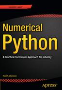
The purpose of storing numerical data in arrays is to be able to process the data with concise vectorized expressions that represent batch operations that are applied to all elements in the arrays. Efficient use of vectorized expressions eliminates the need of many explicit for loops. This results in less verbose code, better maintainability, and higher-performing code. NumPy implements functions and vectorized operations corresponding to most fundamental mathematical functions and operators. Many of these functions and operations act on arrays on an elementwise basis, and binary operations require all arrays in an expression to be of compatible size. The meaning of compatible size is normally that the variables in an expression represent either scalars or arrays of the same size and shape. More generally, a binary operation involving two arrays is well defined if the arrays can be broadcasted into the same shape and size.
In the case of an operation between a scalar and an array, broadcasting refers to the scalar being distributed and the operation applied to each element in the array. When an expression contains arrays of unequal size, the operations may still be well-defined if the smaller of the array can be broadcasted (“effectively expanded”) to match the larger array according to NumPy’s broadcasting rule: An array can be broadcasted over another array if their axes on a one-by-one basis either have the same length or if either of them have length 1. If the number of axes of the two arrays is not equal, the array with fewer axes is padded with new axes of length 1 from the left until the numbers of dimensions of the two arrays agree.
Two simple examples that illustrates array broadcasting is shown in Figure 2-2: A ![]() matrix is added to a
matrix is added to a ![]() row vector and a
row vector and a ![]() column vector, respectively, and the in both cases the result is a
column vector, respectively, and the in both cases the result is a ![]() matrix. However, the elements in the two resulting matrices are different, because the way the elements of the row and column vectors are broadcasted to the shape of the larger array is different depending on the shape of the arrays, according to NumPy’s broadcasting rule.
matrix. However, the elements in the two resulting matrices are different, because the way the elements of the row and column vectors are broadcasted to the shape of the larger array is different depending on the shape of the arrays, according to NumPy’s broadcasting rule.
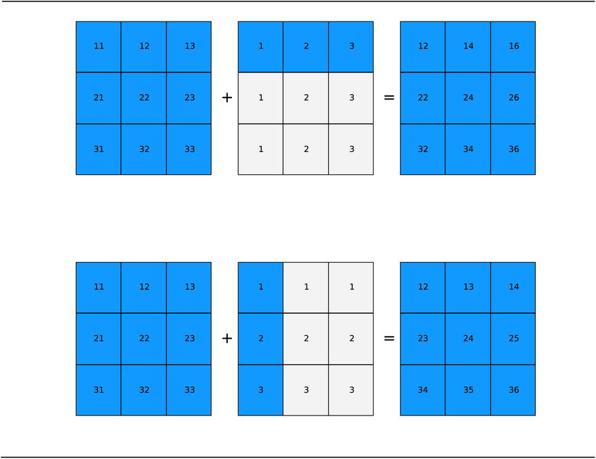
Figure 2-2. Visualization of broadcasting of row and column vectors into the shape of a matrix. The highlighted elements represent true elements of the arrays, while the light gray shaded elements describe the broadcasting of the elements of the array of smaller size
Arithmetic Operations
The standard arithmetic operations with NumPy arrays perform elementwise operations. Consider, for example, the addition, subtraction, multiplication and division of equal-sized arrays:
In [132]: x = np.array([[1, 2], [3, 4]])
In [133]: y = np.array([[5, 6], [7, 8]])
In [134]: x + y
Out[134]: array([[ 6,  8],
                 [10, 12]])
In [135]: y - x
Out[135]: array([[4, 4],
                 [4, 4]])
In [136]: x * y
Out[136]: array([[ 5, 12],
                 [21, 32]])
In [137]: y / x
Out[137]: array([[ 5.        ,  3.        ],
                 [ 2.33333333,  2.        ]])
In operations between scalars and arrays, the scalar value is applied to each element in the array, as one could expect:
In [138]: x * 2
Out[138]: array([[2, 4],
                 [6, 8]])
In [139]: 2 ** x
Out[139]: array([[ 2,  4],
                 [ 8, 16]])
In [140]: y / 2
Out[140]: array([[ 2.5,  3. ],
                 [ 3.5,  4. ]])
In [141]: (y / 2).dtype
Out[141]: dtype('float64')
Note that the dtype of the resulting array for an expression can be promoted if the computation requires it, as shown in the example above with division between an integer array and an integer scalar, which in that case resulted in an array with a dtype that is np.float64.
If an arithmetic operation is performed on arrays with incompatible size or shape, a ValueError exception is raised:
In [142]: x = np.array([1, 2, 3, 4]).reshape(2, 2)
In [143]: z = np.array([1, 2, 3, 4])
In [144]: x / z
---------------------------------------------------------------------------
ValueError                                Traceback (most recent call last)
<ipython-input-144-b88ced08eb6a> in <module>()
----> 1 x / z
ValueError: operands could not be broadcast together with shapes (2,2) (4,)
Here the array x has shape (2, 2) and array z has shape (4,), which cannot be broadcasted into a form that is compatible with (2, 2). If, on the other hand, z has shape (2,), (2, 1), or (1, 2), then it can broadcasted to the shape (2, 2) by effectively repeating the array z along the axis with length 1. Let’s first consider an example with an array z of shape (1, 2), where the first axis (axis 0) has length 1:
In [145]: z = np.array([[2, 4]])
In [146]: z.shape
Out[146]: (1, 2)
Dividing the array x with array z is equivalent to dividing x with an array zz that is constructed by repeating (here using np.concatenate) the row vector z to obtain an array zz that has the same dimensions as x:
In [147]: x / z
Out[147]: array([[ 0.5,  0.5],
                 [ 1.5,  1. ]])
In [148]: zz = np.concatenate([z, z], axis=0)
In [149]: zz
Out[149]: array([[2, 4],
                 [2, 4]])
In [150]: x / zz
Out[150]: array([[ 0.5,  0.5],
                 [ 1.5,  1. ]])
Let’s also consider the example in which the array z has shape (2, 1), and where the second axis (axis 1) has length 1:
In [151]: z = np.array([[2], [4]])
In [152]: z.shape
Out[152]: (2, 1)
In this case, dividing x with z is equivalent to dividing x with an array zz that is constructed by repeating the column vector z until a matrix with same dimension as x is obtained.
In [153]: x / z
Out[153]: array([[ 0.5 ,  1.  ],
                 [ 0.75,  1.  ]])
In [154]: zz = np.concatenate([z, z], axis=1)
In [155]: zz
Out[155]: array([[2, 2],
                 [4, 4]])
In [156]: x / zz
Out[156]: array([[ 0.5 ,  1.  ],
                 [ 0.75,  1.  ]])
In summary, these examples show how arrays with shape (1, 2) and (2, 1) are broadcasted to the shape (2, 2) of the array x when the operation x / z is performed. In both cases, the result of the operation x / z is the same as first repeating the smaller array z along its axis of length 1 to obtain a new array zz with the same shape as x, and then perform the equal-size array operation x / zz. However, the implementation of the broadcasting does not explicitly perform this expansion and the corresponding memory copies, but it can be helpful to think of the array broadcasting in these terms.
A summary of the operators for arithmetic operations with NumPy arrays is given in Table 2-6. These operators use the standard symbols used in Python. The result of an arithmetic operation with one or two arrays is a new independent array, with its own data in the memory. Evaluating a complicated arithmetic expression might therefore trigger many memory allocation and copy operations, and when working with large arrays this can lead to a large memory footprint, and impact the performance negatively. In such cases, using in-place operation (see Table 2-6.) can reduce the memory footprint and improve performance. As an example of in-place operators, consider the following two statements, which have the same effect:
In [157]: x = x + y
In [158]: x += y
The two expressions have the same effect, but in the first case x is reassigned to a new array, while in the second case the values of array x are updated in place. Extensive use of in-place operators tends to impair code readability, and in-place operators should therefore be used only when necessary.
Table 2-6. Operators for elementwise arithmetic operation on NumPy arrays
|
Operator |
Operation |
|---|---|
|
+, += |
Addition |
|
-, -= |
Subtraction |
|
*, *= |
Multiplication |
|
/, /= |
Division |
|
//, //= |
Integer division |
|
**, **= |
Exponentiation |
Elementwise Functions
In addition to arithmetic expressions using operators, NumPy provides vectorized functions for elementwise evaluation of many elementary mathematical functions and operations. Table 2-7 gives a summary of elementary mathematical functions in NumPy.3 Each of these functions takes a single array (of arbitrary dimension) as input and returns a new array of the same shape, where for each element the function has been applied to the corresponding element in the input array. The data type of the output array is not necessarily the same as that of the input array.
Table 2-7. Selection of NumPy functions for elementwise elementary mathematical functions
|
NumPy function |
Description |
|---|---|
|
np.cos, np.sin, np.tan |
Trigonometric functions. |
|
np.arccos, np.arcsin. np.arctan |
Inverse trigonometric functions. |
|
np.cosh, np.sinh, np.tanh |
Hyperbolic trigonometric functions. |
|
np.arccosh, np.arcsinh, np.arctanh |
Inverse hyperbolic trigonometric functions. |
|
np.sqrt |
Square root. |
|
np.exp |
Exponential. |
|
np.log, np.log2, np.log10 |
Logarithms of base e, 2, and 10, respectively. |
For example, the np.sin function (which takes only one argument) is used to compute the sine function for all values in the array:
In [159]: x = np.linspace(-1, 1, 11)
In [160]: x
Out[160]: array([-1. , -0.8, -0.6, -0.4, -0.2,  0. ,  0.2,  0.4,  0.6,  0.8,  1.])
In [161]: y = np.sin(np.pi * x)
In [162]: np.round(y, decimals=4)
Out[162]: array([-0., -0.5878, -0.9511, -0.9511, -0.5878, 0., 0.5878, 0.9511, 0.9511, 0.5878,
0.])
Here we also used the constant np.pi and the function np.round to round the values of y to four decimals. Like the np.sin function, many of the elementary math functions take one input array and produce one output array. In contrast, many of the mathematical operator functions (Table 2-8) operates on two input arrays and returns one array:
In [163]: np.add(np.sin(x) ** 2, np.cos(x) ** 2)
Out[163]: array([ 1.,  1.,  1.,  1.,  1.,  1.,  1.,  1.,  1.,  1.,  1.])
In [164]: np.sin(x) ** 2 + np.cos(x) ** 2
Out[164]: array([ 1.,  1.,  1.,  1.,  1.,  1.,  1.,  1.,  1.,  1.,  1.])
Table 2-8. Summary of NumPy functions for elementwise mathematical operations
|
NumPy function |
Description |
|---|---|
|
np.add, np.subtract, np.multiply, np.divide |
Addition, subtraction, multiplication and division of two NumPy arrays. |
|
np.power |
Raise first input argument to the power of the second input argument (applied elementwise). |
|
np.remainder |
The remainder of division. |
|
np.reciprocal |
The reciprocal (inverse) of each element. |
|
np.real, np.imag, np.conj |
The real part, imaginary part, and the complex conjugate of the elements in the input arrays. |
|
np.sign, np.abs |
The sign and the absolute value. |
|
np.floor, np.ceil, np.rint |
Convert to integer values. |
|
np.round |
Round to a given number of decimals. |
Note that in this example, using np.add and the operator + are equivalent, and for normal use the operator should be used.
Occasionally it is necessary to define new functions that operate on NumPy arrays on an element-by-element basis. A good way to implement such functions is to express it in terms of already existing NumPy operators and expressions, but in cases when this is not possible, the np.vectorize function can be a convenient tool. This function takes a non-vectorized function and returns a vectorized function. For example, consider the following implementation of the Heaviside step function, which works for scalar input:
In [165]: def heaviside(x):
     ...:     return 1 if x > 0 else 0
In [166]: heaviside(-1)
Out[166]: 0
In [167]: heaviside(1.5)
Out[167]: 1
However, unfortunately this function does not work for NumPy array input:
In [168]: x = np.linspace(-5, 5, 11)
In [169]: heaviside(x)
...
ValueError: The truth value of an array with more than one element is ambiguous. Use a.any() or a.all()
Using np.vectorize the scalar heaviside function can be converted into a vectorized function that works with NumPy arrays as input:
In [170]: heaviside = np.vectorize(heaviside)
In [171]: heaviside(x)
Out[171]: array([0, 0, 0, 0, 0, 0, 1, 1, 1, 1, 1])
Although the function returned by np.vectorize works with arrays, it will be relatively slow since the original function must be called for each element in the array. There are much better ways to implementing this particular function using arithmetic with Boolean-valued arrays, as discussed later in this chapter:
In [172]: def heaviside(x):
     ...:     return 1.0 * (x > 0)
Nonetheless, np.vectorize can often be a quick and convenient way to vectorize a function written for scalar input.
In addition to NumPy’s functions for elementary mathematical function, as summarized in Table 2-7, there are also a numerous functions in NumPy for mathematical operations. A summary of a selection of these functions is given in Table 2-8.
Aggregate Functions
NumPy provides another set of functions for calculating aggregates for NumPy arrays, which take an array as input and by default return a scalar as output. For example, statistics such as averages, standard deviations, and variances of the values in the input array, and functions for calculating the sum and the product of elements in an array, are all aggregate functions.
A summary of aggregate functions is given in Table 2-9. All of these functions are also available as methods in the ndarray class. For example, np.mean(data) and data.mean() in the following example are equivalent:
In [173]: data = np.random.normal(size=(15, 15))
In [174]: np.mean(data)
Out[174]: -0.032423651106794522
In [175]: data.mean()
Out[175]: -0.032423651106794522
Table 2-9. NumPy functions for calculating aggregrates of NumPy arrays
|
NumPy Function |
Description |
|---|---|
|
np.mean |
The average of all values in the array. |
|
np.std |
Standard deviation. |
|
np.var |
Variance. |
|
np.sum |
Sum of all elements. |
|
np.prod |
Product of all elements. |
|
np.cumsum |
Cumulative sum of all elements. |
|
np.cumprod |
Cumulative product of all elements. |
|
np.min, np.max |
The minimum / maximum value in an array. |
|
np.argmin, np.argmax |
The index of the minimum / maximum value in an array. |
|
np.all |
Return True if all elements in the argument array are nonzero. |
|
np.any |
Return True if any of the elements in the argument array is nonzero. |
By default, the functions in Table 2-9 aggregate over the entire input array. Using the axis keyword argument with these functions, and their corresponding ndarray methods, it is possible to control over which axis in the array aggregation is carried out. The axis argument can be an integer, which specifies the axis to aggregate values over. In many cases the axis argument can also be a tuple of integers, which specifies multiple axes to aggregate over. The following example demonstrates how calling the aggregate function np.sum on the array of shape (5, 10, 15) reduces the dimensionality of the array depending of the values of the axis argument:
In [176]: data = np.random.normal(size=(5, 10, 15))
In [177]: data.sum(axis=0).shape
Out[177]: (10, 15)
In [178]: data.sum(axis=(0, 2)).shape
Out[178]: (10,)
In [179]: data.sum()
Out[179]: -31.983793284860798
A visual illustration of how aggregation over all elements, over the first axis, and over the second axis of a ![]() array is shown in Figure 2-3. In this example, the data array is filled with integers between 1 and 9:
array is shown in Figure 2-3. In this example, the data array is filled with integers between 1 and 9:
In [180]: data = np.arange(1,10).reshape(3,3)
In [181]: data
Out[181]: array([[1, 2, 3],
                 [4, 5, 6],
                 [7, 8, 9]])
and we compute the aggregate sum of the entire array, over the axis 0, and over axis 1, respectively:
In [182]: data.sum()
Out[182]: 45
In [183]: data.sum(axis=0)
Out[183]: array([12, 15, 18])
In [184]: data.sum(axis=1)
Out[184]: array([ 6, 15, 24])

Figure 2-3. Illustration of array aggregation functions along all axes (left), first axis (center), and the second axis (right) of a two-dimensional array of shape ![]()
Boolean Arrays and Conditional Expressions
When computing with NumPy arrays, there is often a need to compare elements in different arrays, and perform conditional computations based on the results of such comparisons. Like with arithmetic operators, NumPy arrays can be used with the usual comparison operators, for example >, <, >=, <=, == and !=, and the comparisons are made on an element-by-element basis. The broadcasting rules also applies to comparison operators, and if two operators have compatible shapes and sizes, the result of the comparison is a new array with Boolean values (with dtype as np.bool) that gives the result of the comparison for each element:
In [185]: a = np.array([1, 2, 3, 4])
In [186]: b = np.array([4, 3, 2, 1])
In [187]: a < b
Out[187]: array([ True,  True, False, False], dtype=bool)
To use the result of a comparison between arrays in for example an if statement, we need to aggregate the Boolean values of the resulting arrays in some suitable fashion, to obtain a single True or False value. A common use-case is to apply the np.all or np.any aggregation functions, depending on the situation at hand:
In [188]: np.all(a < b)
Out[188]: False
In [189]: np.any(a < b)
Out[189]: True
In [190]: if np.all(a < b):
     ...:     print("All elements in a are smaller than their corresponding element in b")
     ...: elif np.any(a < b):
     ...:     print("Some elements in a are smaller than their corresponding elemment in b")
     ...: else:
     ...:     print("All elements in b are smaller than their corresponding element in a")
Some elements in a are smaller than their corresponding elemment in b
The advantage of Boolean-valued arrays, however, is that they often make it possible to avoid conditional if statements altogether. By using Boolean-valued arrays in arithmetic expressions, it is possible to write conditional computations in vectorized form. When appearing in an arithmetic expression together with a scalar number, or another NumPy array with a numerical data type, a Boolean array is converted to a numerical-valued array with values 0 and 1 in place of False and True, respectively.
In [191]: x = np.array([-2, -1, 0, 1, 2])
In [192]: x > 0
Out[192]: array([False, False, False,  True,  True], dtype=bool)
In [193]: 1 * (x > 0)
Out[193]: array([0, 0, 0, 1, 1])
In [194]: x * (x > 0)
Out[194]: array([0, 0, 0, 1, 2])
This is a useful property for conditional computing, such as when defining piecewise functions. For example, if we need to define a function describing a pulse of given height, width and position, we can implement this function by multiplying the height (a scalar variable) with two Boolean-valued arrays for the spatial extension of the pulse:
In [195]: def pulse(x, position, height, width):
     ...:     return height * (x >= position) * (x <= (position + width))
In [196]: x = np.linspace(-5, 5, 11)
In [197]: pulse(x, position=-2, height=1, width=5)
Out[197]: array([0, 0, 0, 1, 1, 1, 1, 1, 1, 0, 0])
In [198]: pulse(x, position=1, height=1, width=5)
Out[198]: array([0, 0, 0, 0, 0, 0, 1, 1, 1, 1, 1])
In this example, the expression (x >= position) * (x <= (position + width)) is a multiplication of two Boolean-valued arrays, and for this case the multiplication operator act as an elementwise AND operator. The function pulse could also be implemented using NumPy’s function for elementwise AND operations, np.logical_and:
In [199]: def pulse(x, position, height, width):
     ...:     return height * np.logical_and(x >= position, x <= (position + width))
There are also functions for other logical operations, such as NOT, OR and XOR, and functions for selectively picking values from different arrays depending on a given condition np.where, list of conditions np.select, and an array of indices np.choose. See Table 2-10 for a summary of such functions, and the following examples demonstrate the basic usage of some of these functions. The np.where function selects elements from two arrays (second and third arguments), given a Boolean-valued array condition (the first argument). For elements where the condition is True, the corresponding values from the array given as second argument are selected, and if the condition is False, elements from the third argument array are selected:
In [200]: x = np.linspace(-4, 4, 9)
In [201]: np.where(x < 0, x**2, x**3)
Out[201]: array([ 16.,   9.,   4.,   1.,   0.,   1.,   8.,  27.,  64.])
Table 2-10. NumPy functions for conditional and logical expressions
|
Function |
Description |
|---|---|
|
np.where |
Choose values from two arrays depending on the value of a condition array. |
|
np.choose |
Choose values from a list of arrays depending on the values of a given index array. |
|
np.select |
Choose values from a list of arrays depending on a list of conditions. |
|
np.nonzero |
Return an array with indices of nonzero elements. |
|
np.logical_and |
Perform and elementwise AND operation. |
|
np.logical_or, np.logical_xor |
Elementwise OR/XOR operations. |
|
np.logical_not |
Elementwise NOT operation (inverting). |
The np.select function works similarly, but instead of a Boolean-valued condition array it expects a list of Boolean-valued condition arrays, and a corresponding list of value arrays:
In [202]: np.select([x < -1, x < 2, x >= 2],
     ...:           [x**2  , x**3 , x**4])
Out[202]: array([  16.,    9.,    4.,   -1.,    0.,    1.,   16.,   81.,  256.])
The np.choose takes as a first argument a list or an array with indices that determine from which array in a given list of arrays an element is picked from:
In [203]: np.choose([0, 0, 0, 1, 1, 1, 2, 2, 2],
     ...:           [x**2,  x**3,  x**4])
Out[203]: array([  16.,    9.,    4.,   -1.,    0.,    1.,   16.,   81.,  256.])
The function np.nonzero returns a tuple of indices that can be used to index the array (for example the one that the condition was based on). This has the same results as indexing the array directly with abs(x) > 2, but it uses fancy indexing with the indices returned by np.nonzero rather than Boolean-valued array indexing.
In [204]: np.nonzero(abs(x) > 2)
Out[204]: (array([0, 1, 7, 8]),)
In [205]: x[np.nonzero(abs(x) > 2)]
Out[205]: array([-4., -3.,  3.,  4.])
In [206]: x[abs(x) > 2]
Out[206]: array([-4., -3.,  3.,  4.])
Set Operations
The Python language provides a convenient set data structure for managing unordered collections of unique objects. The NumPy array class ndarray can also be used to describe such sets, and NumPy contains functions for operating on sets stored as NumPy arrays. These functions are summarized in Table 2-11. Using NumPy arrays to describe and operate on sets allows expressing certain operations in vectorized form. For example, testing if the values in a NumPy array are included in a set can be done using the np.in1d function, which tests for the existence of each element of its first argument in the array passed as second argument. To see how this works, consider the follow example: first, to ensure that a NumPy array is a proper set, we can use the np.unique function, which returns a new array with unique values:
In [207]: a = np.unique([1, 2, 3, 3])
In [208]: b = np.unique([2, 3, 4, 4, 5, 6, 5])
In [209]: np.in1d(a, b)
Out[209]: array([False,  True,  True], dtype=bool)
Here, the existence of each element in a in the set b was tested, and the result is a Boolean-valued array. Note that we can use the in keyword to test for the existence of single elements in a set represented as NumPy array:
In [210]: 1 in a
Out[210]: True
In [211]: 1 in b
Out[211]: False
To test if a is a subset of b, we can use the np.in1d, as in the previous example, together with the aggregation function np.all (or the corresponding ndarray method):
In [212]: np.all(np.in1d(a, b))
Out[212]: False
The standard set operations union (the set of elements included in either or both sets), intersection (elements included in both sets), and difference (elements included in one of the sets but not the other) are provided by np.union1d, np.intersect1d, and np.setdiff1d, respectively:
In [213]: np.union1d(a, b)
Out[213]: array([1, 2, 3, 4, 5, 6])
In [214]: np.intersect1d(a, b)
Out[214]: array([2, 3])
In [215]: np.setdiff1d(a, b)
Out[215]: array([1])
In [216]: np.setdiff1d(b, a)
Out[216]: array([4, 5, 6])
Table 2-11. NumPy functions for operating on sets
|
Function |
Description |
|---|---|
|
np.unique |
Create a new array with unique elements, where each value only appears once. |
|
np.in1d |
Test for the existence of an array of elements in another array. |
|
np.intersect1d |
Return an array with elements that are contained in two given arrays. |
|
np.setdiff1d |
Return an array with elements that are contained in one but not the other, of two given arrays. |
|
np.union1d |
Return an array with elements that are contained in either, or both, of two given arrays. |
Operations on Arrays
In addition to elementwise and aggregation functions, some operations act on arrays as a whole, and produce transformed array of the same size. An example of this type of operation is the transpose, which flips the order of the axes of an array. For the special case of a two-dimensional array, that is, a matrix, the transpose simply exchanges rows and columns:
In [217]: data = np.arange(9).reshape(3, 3)
In [218]: data
Out[218]: array([[0, 1, 2],
                 [3, 4, 5],
                 [6, 7, 8]])
In [219]: np.transpose(data)
Out[219]: array([[0, 3, 6],
                 [1, 4, 7],
                 [2, 5, 8]])
The transpose function np.transpose also exists as a method in ndarray, and as the special method name ndarray.T. For an arbitrary N-dimensional array, the transpose operation reverses all the axes, as can be seen from the following example (note that here the shape attribute is used to display the number of values along each axis of the array):
In [220]: data = np.random.randn(1, 2, 3, 4, 5)
In [221]: data.shape
Out[221]: (1, 2, 3, 4, 5)
In [222]: data.T.shape
Out[222]: (5, 4, 3, 2, 1)
The np.fliplr (flip left-right) and np.flipud (flip up-down) functions perform operations that are similar to the transpose: they reshuffle the elements of an array so that the elements in rows (np.fliplr) or columns (np.flipud) are reversed, and the shape of the output array is the same as the input. The np.rot90 function rotates the elements in the first two axes in an array by 90 degrees, and like the transpose function it can change the shape of the array. Table 2-12 gives a summary of NumPy functions for common array operations.
Table 2-12. Summary of NumPy functions for array operations
|
Function |
Description |
|---|---|
|
np.transpose, np.ndarray.transpose, np.ndarray.T |
The transpose (reverse axes) of an array. |
|
np.fliplr / np.flipud |
Reverse the elements in each row / column. |
|
np.rot90 |
Rotate the elements along the first two axes by 90 degrees. |
|
np.sort, np.ndarray.sort |
Sort the element of an array along a given specified axis (which default to the last axis of the array). The np.ndarray method sort performs the sorting in place, modifying the input array. |
Matrix and Vector Operations
We have so far discussed general N-dimensional arrays. One of the main applications of such arrays is to represent the mathematical concepts of vectors, matrices, and tensors, and in this use-case we also frequently need to calculate vector and matrix operations such as scalar (inner) products, dot (matrix) products, and tensor (outer) products. A summary of NumPy’s functions for matrix operations is given in Table 2-13.
Table 2-13. Summary of NumPy functions for matrix operations
|
NumPy Function |
Description |
|---|---|
|
np.dot |
Matrix multiplication (dot product) between two given arrays representing vectors, arrays, or tensors. |
|
np.inner |
Scalar multiplication (inner product) between two arrays representing vectors. |
|
np.cross |
The cross product between two arrays that represent vectors. |
|
np.tensordot |
Dot product along specified axes of multidimensional arrays. |
|
np.outer |
Outer product (tensor product of vectors) between two arrays representing vectors. |
|
np.kron |
Kronecker product (tensor product of matrices) between arrays representing matrices and higher-dimensional arrays. |
|
np.einsum |
Evaluates Einstein’s summation convention for multidimensional arrays. |
In NumPy, the * operator is used for elementwise multiplication. For two two-dimensional arrays A and B, the expression A * B therefore does not compute a matrix product (in contrast to many other computing environments). Currently there is no operator for denoting matrix multiplication,4 and instead the NumPy function np.dot is used for this purpose. There is also a corresponding method in the ndarray class. To compute the product of two matrices A and B, of size ![]() and
and ![]() , which results in a matrix of size
, which results in a matrix of size ![]() , we can use:
, we can use:
In [223]: A = np.arange(1, 7).reshape(2, 3)
In [224]: A
Out[224]: array([[1, 2, 3],
                 [4, 5, 6]])
In [225]: B = np.arange(1, 7).reshape(3, 2)
In [226]: B
Out[226]: array([[1, 2],
                 [3, 4],
                 [5, 6]])
In [227]: np.dot(A, B)
Out[227]: array([[22, 28],
                 [49, 64]])
In [228]: np.dot(B, A)
Out[228]: array([[ 9, 12, 15],
                 [19, 26, 33],
                 [29, 40, 51]])
The np.dot function is also be used for matrix-vector multiplication (that is, multiplication of a two-dimension array, that represent a matrix, with a one-dimensional array representing a vector). For example:
In [229]: A = np.arange(9).reshape(3, 3)
In [230]: A
Out[230]: array([[0, 1, 2],
                 [3, 4, 5],
                 [6, 7, 8]])
In [231]: x = np.arange(3)
In [232]: x
Out[232]: array([0, 1, 2])
In [233]: np.dot(A, x)
Out[233]: array([5, 14, 23])
In this example, x can be either a two-dimensional array of shape (1, 3) or a one-dimensional array with shape (3,). In addition to the function np.dot, there is also a corresponding method dot in ndarray, which can be used as in the following example:
In [234]: A.dot(x)
Out[234]: array([5, 14, 23])
Unfortunately, nontrivial matrix multiplication expressions can often become complex and hard to read when using either np.dot or np.ndarray.dot. For example, even a relatively simple matrix expression like the one for a similarity transform, ![]() , must be represented with relatively cryptic nested expressions,5 such as either
, must be represented with relatively cryptic nested expressions,5 such as either
In [235]: A = np.random.rand(3, 3)
In [236]: B = np.random.rand(3, 3)
In [237]: Ap = np.dot(B, np.dot(A, np.linalg.inv(B)))
or
In [238]: Ap = B.dot(A.dot(np.linalg.inv(B)))
To improve this situation, NumPy provides an alternative data structure to ndarray named matrix, for which expressions like A * B are implemented as matrix multiplication. It also provides some convenient special attributes, like matrix.I for the inverse matrix, and matrix.H for the complex-conjugate transpose of a matrix. Using instances of this matrix class, one can therefore use the vastly more readable expression:
In [239]: A = np.matrix(A)
In [240]: B = np.matrix(B)
In [241]: Ap = B * A * B.I
This may seem like a practical compromise, but unfortunately using the matrix class does have a few disadvantages, and its use is therefore often discouraged. The main objection against using matrix is that expression like A * B are then context dependent: that is, it is not immediately clear if A * B denotes elementwise or matrix multiplication, because it depends on the type of A and B, and this creates another code-readability problem. This can be a particularly relevant issue if A and B are user-supplied arguments to a function, in which case it would be necessary to cast all input arrays explicitly to matrix instances, using, for example, np.asmatrix or the function np.matrix (since there would be no guarantee that the user calls the function with arguments of type matrix rather than ndarray). The np.asmatrix function creates a view of the original array in the form of an np.matrix instance. This does not add much in computational costs, but explicitly casting arrays back and forth between ndarray and matrix does offset much of the benefits of the improved readability of matrix expressions. A related issue is that some functions that operate on arrays and matrices might not respect the type of the input, and may return an ndarray even though it was called with an input argument of type matrix. This way, a matrix of type matrix might be unintentionally converted to ndarray, which in turn would change the behavior of expressions like A * B. This type of behavior is not likely to occur when using NumPy’s array and matrix functions, but it is not unlikely to happen when using functions from other packages. However, in spite of all the arguments for not using matrix matrices too extensively, personally I think that using matrix class instances for complicated matrix expressions is an important use-case, and in these cases it might be a good idea to explicitly cast arrays to matrices before the computation, and explicitly cast the result back to the ndarray type, following the pattern:
In [242]: A = np.asmatrix(A)
In [243]: B = np.asmatrix(B)
In [244]: Ap = B * A * B.I
In [245]: Ap = np.asarray(Ap)
The inner product (scalar product) between two arrays representing vectors can be computed using the np.inner function:
In [246]: np.inner(x, x)
Out[246]: 5
or, equivalently, using np.dot:
In [247]: np.dot(x, x)
Out[247]: 5
The main difference is that np.inner expects two input arguments with the same dimension, while np.dot can take input vectors of shape ![]() and
and ![]() , respectively:
, respectively:
In [248]: y = x[:, np.newaxis]
In [249]: y
Out[249]: array([[0],
                 [1],
                 [2]])
In [250]: np.dot(y.T, y)
Out[250]: array([[5]])
While the inner product maps two vectors to a scalar, the outer product performs the complementary operation of mapping two vectors to a matrix.
In [251]: x = np.array([1, 2, 3])
In [252]: np.outer(x, x)
Out[252]: array([[1, 2, 3],
                 [2, 4, 6],
                 [3, 6, 9]])
The outer product can also be calculated using the Kronecker product using the function np.kron, which, however, in contrast to np.outer, produce an output array of shape (M*P, N*Q) if the input arrays have shapes (M, N) and (P, Q), respectively. Thus, for the case of two one-dimensional arrays of length M and P, the resulting array has shape (M*P,):
In [253]: np.kron(x, x)
Out[253]: array([1, 2, 3, 2, 4, 6, 3, 6, 9])
To obtain the result that corresponds to np.outer(x, x), the input array x must be expanded to shape (N, 1) and (1, N), in the first and second argument to np.kron, respectively:
In [254]: np.kron(x[:, np.newaxis], x[np.newaxis, :])
Out[254]: array([[1, 2, 3],
                 [2, 4, 6],
                 [3, 6, 9]])
In general, while the np.outer function is primarily intended for vectors as input, the np.kron function can be used for computing tensor products of arrays of arbitrary dimension (but both inputs must have the same number of axes). For example, to compute the tensor product of two ![]() matrices, we can use:
matrices, we can use:
In [255]: np.kron(np.ones((2,2)), np.identity(2))
Out[255]: array([[ 1.,  0.,  1.,  0.],
                 [ 0.,  1.,  0.,  1.],
                 [ 1.,  0.,  1.,  0.],
                 [ 0.,  1.,  0.,  1.]])
In [256]: np.kron(np.identity(2), np.ones((2,2)))
Out[256]: array([[ 1.,  1.,  0.,  0.],
                 [ 1.,  1.,  0.,  0.],
                 [ 0.,  0.,  1.,  1.],
                 [ 0.,  0.,  1.,  1.]])
When working with multidimensional arrays it is often possible to express common array operations concisely using Einstein’s summation convention, in which an implicit summation is assumed over each index that occurs multiple times in an expression. For example, the scalar product between two vectors x and y can is compactly expressed as xnyn and the matrix multiplication of two matrices A and B is expressed as AmkBkn. NumPy provides the function np.einsum for carrying out Einstein summations. Its first argument is an index expression, followed by an arbitrary number of arrays that are included in the expression. The index expression is a string with comma-separated indices, where each comma separates the indices of each array. Each array can have any number of indices. For example, the scalar product expression xn yn can be evaluated with np.einsum using the index expression "n,n", that is using np.einsum("n,n", x, y):
In [257]: x = np.array([1, 2, 3, 4])
In [258]: y = np.array([5, 6, 7, 8])
In [259]: np.einsum("n,n", x, y)
Out[259]: 70
In [260]: np.inner(x, y)
Out[260]: 70
Similarly, the matrix multiplication Amk Bkn can be evaluated using np.einsum and the index expression "mk,kn":
In [261]: A = np.arange(9).reshape(3, 3)
In [262]: B = A.T
In [263]: np.einsum("mk,kn", A, B)
Out[263]: array([[  5,  14,  23],
                 [ 14,  50,  86],
                 [ 23,  86, 149]])
In [264]: np.alltrue(np.einsum("mk,kn", A, B) == np.dot(A, B))
Out[264]: True
The Einstein summation convention can be particularly convenient when dealing with multidimensional arrays, since the index expression that defines the operation makes it explicit which operation is carried out, and along which axes it is performed. An equivalent computation using, for example, np.tensordot might require giving the axes along which the dot product is to be evaluated.
Summary
In this chapter we have given a brief introduction to array-based programming with the NumPy library that can serve as a reference for the following chapters in this book. NumPy is a core library for computing with Python that provides a foundation for nearly all computational libraries for Python. Familiarity with the NumPy library and its usage patterns is a fundamental skill for using Python for scientific and technical computing. Here we started with introducing NumPy’s data structure for n-dimensional arrays – the ndarray object – and we continued by discussing functions for creating and manipulating arrays, including indexing and slicing for extracting elements from arrays. We also discussed functions and operators for performing computations with ndarray objects, with an emphasis on vectorized expressions and operators for efficient computation with arrays. Throughout the rest of this book we will see examples of higher-level libraries for specific fields in scientific computing that use the array framework provided by NumPy.
Further Reading
The NumPy library is the topic of several books, including the Guide to NumPy, by the creator of the NumPy T. Oliphant, available for free online at http://web.mit.edu/dvp/Public/numpybook.pdf, and a series of books by Ivan Idris and one by Wes McKinney.
References
Idris, I. (2012). NumPy Cookbook. Mumbai: Packt.
Idris, I. (2014). Learning NumPy Array. Mumbai: Packt.
Idris, I. (2015). Numpy Beginner's Guide. 3rd ed. Mumbai: Packt.
McKinney, Wes. Python for Data Analysis. Sepastopol: O'Reilly, 2013.
___________________
1Many modern processors provide instructions that operate on arrays. These are also known as vectorized operations, but here vectorized refers to high-level array-based operations, regardless of how they are implemented at the processor level.
2This does not necessarily need to be the case for Python lists, which therefore can be heterogeneous.
3Note that this is not a complete list of the available elementwise functions in NumPy. See the NumPy reference documentation for comprehensive lists.
4Python recently adopted the @ symbol for denoting matrix multiplication. However, at the time of writing, this proposal has not yet been implemented. See http://legacy.python.org/dev/peps/pep-0465 for details.
5With the new proposed infix matrix multiplication operator this same expression could be expressed as the considerably more readable: Ap = B @ A @ np.linalg.inv(B).