
![]()
Signal Processing
In this chapter we explore signal processing, which is a subject with applications in diverse branches of science and engineering. A signal in this context can be a quantity that varies in time (temporal signal), or as a function of space coordinates (spatial signal). For example, an audio signal is a typical example of a temporal signal, while an image is a typical example of a spatial signal in two dimensions. In reality, signals are often continuous functions, but in computational applications it is common to work with discretized signals, where the original continuous signal is sampled at discrete points with uniform distances. The sampling theorem gives rigorous and quantitative conditions for when a continuous signal can be accurately represented by a discrete sequence of samples.
Computational methods for signal processing play a central role in scientific computing not only because of their widespread applications, but also because there exist very efficient computational methods for important signal-processing problems. In particular, the Fast Fourier Transform (FFT) is an important algorithm for many signal-processing problems, and moreover it is perhaps one of the most important numerical algorithms in all of computing. In this chapter we explore how FFTs can be used in spectral analysis, but beyond this basic application there are also broad uses of FFT both directly and indirectly as a component in other algorithms. Other signal-processing methods, such as convolution and correlation analysis, and linear filters also have widespread applications, in particular in engineering fields such as control theory.
In this chapter we discuss spectral analysis and basic applications of linear filters, using the fftpack and signal modules in the SciPy library.
Importing Modules
In this chapter we mainly work with the fftpack and signal modules from the SciPy library. As usual with modules from the SciPy library, we import the modules using the following pattern:
In [1]: from scipy import fftpack
In [2]: from scipy import signal
We also use the io.wavefile module from SciPy to read and write WAV audio files in one of the examples. We import this module in the following way:
In [3]: import scipy.io.wavfile
In [4]: from scipy import io
For basic numerics and graphics we also require the NumPy, Pandas, and Matplotlib libraries:
In [5]: import numpy as np
In [6]: import pandas as pd
In [7]: import matplotlib.pyplot as plt
In [8]: import matplotlib as mpl
Spectral Analysis
We begin this exploration of signal processing by considering spectral analysis. Spectral analysis is a fundamental application of Fourier transforms, which is a mathematical integral transform that allows us to take a signal from the time domain – where it is described as a function of time – to the frequency domain – where it is described as a function of frequency. The frequency domain representation of a signal is useful for many purposes. Examples include the following: extracting features such as dominant frequency components of a signal, applying filters to signals, and for solving differential equations (see Chapter 9), just to mention a few.
Fourier Transforms
The mathematical expression for the Fourier transform F(ν) of a continuous signal f(t) is1
![]()
and the inverse Fourier transform is given by
![]()
Here F (ν) is the complex-valued amplitude spectrum of the signal f (t), and ν is the frequency. From F(ν) we can compute other types of spectrum, such as the power spectrum |F (ν)|2. In this formulation f (t) is a continuous signal with infinite duration. In practical applications we are often more interested in approximating f (t) using a finite number of samples from a finite duration of time. For example, we might sample the function f (t) at N uniformly spaced points in the time interval ![]() , resulting in a sequence of samples that we denote (x0, x1, ... , xN). The continuous Fourier transform shown above can be adapted to the discrete case: The Discrete Fourier Transform (DFT) of a sequence of uniformly spaced samples is
, resulting in a sequence of samples that we denote (x0, x1, ... , xN). The continuous Fourier transform shown above can be adapted to the discrete case: The Discrete Fourier Transform (DFT) of a sequence of uniformly spaced samples is
![]()
and similarly we have the inverse DFT
![]()
where Xk is the discrete Fourier transform of the samples xn, and k is a frequency bin number that can be related to a real frequency. The DFT for a sequence of samples can be computed very efficiently using the algorithm known as Fast Fourier Transform (FFT). The SciPy fftpack module2 provides implementations of the FFT algorithm. The fftpack module contains FFT functions for a variety of cases: See Table 17-1 for a summary. Here we focus on demonstrating the usage of the fft and ifft functions, and several of the helper functions in the fftpack module. However, the general usage is similar for all FFT functions in Table 17-1.
Table 17-1. Summary of selected functions from the fftpack module in SciPy. For detailed usage of each function, including their arguments and return values, see their docstrings that are available using help(fftpack.fft)
|
Function |
Description |
|---|---|
|
fft, ifft |
General FFT and inverse FFT of a real- or complex-valued signal. The resulting frequency spectrum is complex valued. |
|
rfft, irfft |
FFT and inverse FFT of a real-valued signal. |
|
dct, idct |
The discrete cosine transform (DCT) and its inverse. |
|
dst, idst |
The discrete sine transform (DST) and its inverse. |
|
fft2, ifft2, fftn, ifftn |
The 2-dimensional and the n-dimensional FFT for complex-valued signals, and their inverses. |
|
fftshift, ifftshift, rfftshift, irfftshift |
Shift the frequency bins in the result vector produced by fft and rfft, respectively, so that the spectrum is arranged such that the zero-frequency component is in the middle of the array. |
|
fftfreq |
Calculate the frequencies corresponding to the FFT bins in the result returned by fft. |
Note that the DFT takes discrete samples as input, and outputs a discrete frequency spectrum. To be able to use DFT for processes that are originally continuous we first must reduce the signals to discrete values using sampling. According to the sampling theorem, a continuous signal with bandwidth B (that is, the signal does not contain frequencies higher than B), can be completely reconstructed from discrete samples with sampling frequency ![]() . This is a very important result in signal processing, because it tells us under what circumstances we can work with discrete instead of continuous signals. It allows us to determine a suitable sampling rate when measuring a continuous process, since it is often possible to know or approximately guess the bandwidth of a process, for example, from physical arguments. While the sampling rate determines the maximum frequency we can describe with a discrete Fourier transform, the spacing of samples in frequency space is determined by the total sampling time T, or equivalently from the number of samples points once the sampling frequency is determined,
. This is a very important result in signal processing, because it tells us under what circumstances we can work with discrete instead of continuous signals. It allows us to determine a suitable sampling rate when measuring a continuous process, since it is often possible to know or approximately guess the bandwidth of a process, for example, from physical arguments. While the sampling rate determines the maximum frequency we can describe with a discrete Fourier transform, the spacing of samples in frequency space is determined by the total sampling time T, or equivalently from the number of samples points once the sampling frequency is determined, ![]() .
.
As an introductory example, consider a simulated signal with pure sinusoidal components at 1 Hz and at 22 Hz, on top of a normal-distributed noise floor. We begin by defining a function signal_samples that generates noisy samples of this signal:
In [9]: def signal_samples(t):
   ...:     return (2 * np.sin(2 * np.pi * t) + 3 * np.sin(22 * 2 * np.pi * t) +
   ...:             2 * np.random.randn(*np.shape(t)))
We can get a vector of samples from by calling this function with an array with sample times as argument. Say that we are interested in computing the frequency spectrum of this signal up to frequencies of at 30 Hz. We then need to choose the sampling frequency ![]() 60 Hz, and if we want to obtain a frequency spectrum with resolution of
60 Hz, and if we want to obtain a frequency spectrum with resolution of ![]() 0.01 Hz, we need to collect at least
0.01 Hz, we need to collect at least ![]() 6000 samples, corresponding to a sampling period of
6000 samples, corresponding to a sampling period of ![]() 100 seconds:
100 seconds:
In [10]: B = 30.0
In [11]: f_s = 2 * B
In [12]: delta_f = 0.01
In [13]: N = int(f_s / delta_f); N
Out[13]: 6000
In [14]: T = N / f_s; T
Out[14]: 100.0
Next we sample the signal function at N uniformly spaced points in time by first creating an array t that contains the sample times, and then use it to evaluate the signal_samples function:
In [15]: t = np.linspace(0, T, N)
In [16]: f_t = signal_samples(t)
The resulting signal is plotted in Figure 17-1. The signal is rather noisy, both when viewed over the entire sampling time, and when viewed for a shorter period of time, and the added random noise mostly masks the pure sinusoidal signals when viewed in time domain.
In [17]: fig, axes = plt.subplots(1, 2, figsize=(8, 3), sharey=True)
    ...: axes[0].plot(t, f_t)
    ...: axes[0].set_xlabel("time (s)")
    ...: axes[0].set_ylabel("signal")
    ...: axes[1].plot(t, f_t)
    ...: axes[1].set_xlim(0, 5)
    ...: axes[1].set_xlabel("time (s)")
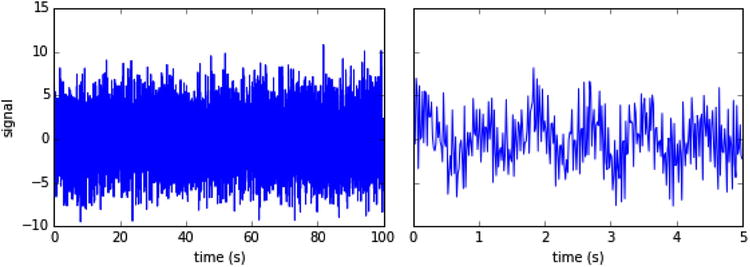
Figure 17-1. Simulated signal with random noise. Full signal to the left, and zoom in to early times on the right
To reveal the sinusoidal components in the signal we can use the FFT to compute the spectrum of the signal (or in order words, its frequency domain representation). We obtain the discrete Fourier transform of the signal by applying the fft function to the array of discrete samples, f_t:
In [18]: F = fftpack.fft(f_t)
The result is an array F, which contains the frequency components of the spectrum at frequencies that are given by the sampling rate and number of samples. When computing these frequencies, it is convenient to use the helper function fftfreq, which takes the number of samples and the time duration between successive samples as parameters, and return an array of the same size as F that contains the frequencies corresponding to each frequency bin.
In [19]: f = fftpack.fftfreq(N, 1.0/f_s)
The frequency bins for the amplitude values returned by the fft function contains both positive and negative frequencies, up to the frequency that corresponds to half the sampling rate, fs/2. For real-valued singals, the spectrum is symmetric at positive and negative frequencies, and we are for this reason often only interested in the positive-frequency components. Using the frequency array f, we can conveniently create a mask that can be used to extract the part of the spectrum that corresponds to the frequencies we are interested in. Here we create a mask for selecting the positive-frequency components:
In [20]: mask = np.where(f >= 0)
The spectrum for the positive-frequency components is shown in Figure 17-2. The top panel contains the entire positive-frequency spectrum, and is plotted on a log scale to increase the contrast between the signal and the noise. We can see that there are sharp peaks near 1 Hz and 22 Hz, corresponding to the sinusoidal components in the signal. These peaks clearly stand out from the noise floor in the spectrum. In spite of the noise concealing the sinusoidal components in the time-domain signal, we can clearly detect their presence in the frequency domain representation. The lower two panels in Figure 17-2 show magnifications of the two peaks at 1 Hz and 22 Hz, respectively.
In [21]: fig, axes = plt.subplots(3, 1, figsize=(8, 6))
    ...: axes[0].plot(f[mask], np.log(abs(F[mask])), label="real")
    ...: axes[0].plot(B, 0, 'r*', markersize=10)
    ...: axes[0].set_ylabel("$log(|F|)$", fontsize=14)
    ...: axes[1].plot(f[mask], abs(F[mask])/N, label="real")
    ...: axes[1].set_xlim(0, 2)
    ...: axes[1].set_ylabel("$|F|$", fontsize=14)
    ...: axes[2].plot(f[mask], abs(F[mask])/N, label="real")
    ...: axes[2].set_xlim(21, 23)
    ...: axes[2].set_xlabel("frequency (Hz)", fontsize=14)
    ...: axes[2].set_ylabel("$|F|$", fontsize=14)

Figure 17-2. Spectrum of the simulated signal with frequency components at 1 Hz and 22 Hz
Frequency-domain Filter
Just like we can compute the frequency-domain representation from the time-domain signal using the FFT function fft, we can compute the time domain signal from the frequency-domain representation using the inverse FFT function ifft. For example, applying the ifft function to the F array will reconstruct the f_t array. By modifying the spectrum before we apply the inverse transform we can realize frequency-domain filters. For example, selecting only frequencies below 2 Hz in the spectrum amounts to applying a 2 Hz low-pass filter, which suppresses high-frequency components in the signal (higher than 2 Hz in this case):
In [22]: F_filtered = F * (abs(f) < 2)
In [23]: f_t_filtered = fftpack.ifft(F_filtered)
Computing the inverse FFT for the filtered signal results in a time-domain signal where the high-frequency oscillations are absent, as shown in Figure 17-3. This simple example summarizes the essence of many frequency-domain filters. Later in this chapter we explore in more detail some of the many types of filters that are commonly used in signal-processing analysis.
In [24]: fig, ax = plt.subplots(figsize=(8, 3))
    ...: ax.plot(t, f_t, label='original')
    ...: ax.plot(t, f_t_filtered.real, color="red", lw=3, label='filtered')
    ...: ax.set_xlim(0, 10)
    ...: ax.set_xlabel("time (s)")
    ...: ax.set_ylabel("signal")
    ...: ax.legend()

Figure 17-3. The original time-domain signal and the reconstructed signal after applying a low-pass filter to the frequency domain representation of the signal
Windowing
In the previous section we directly applied the FFT to the signal. This can give acceptable results, but it is often possible to further improve the quality and the contrast of the frequency spectrum by applying a so-called window function to the signal before applying the FFT. A window function is a function that when multiplied with the signal modulates its magnitude so that it approaches zero at the beginning and the end of the sampling duration. There are many possible functions that can be used as window function, and the SciPy signal module provides implementations of many common window functions, including the Blackman function, the Hann function, the Hamming function, Gaussian window functions (with variable standard deviation), and the Kaiser window function.3 These functions are all plotted in Figure 17-4. This graph shows that while all of these window functions are slightly different, the overall shape is very similar.
In [25]: fig, ax = plt.subplots(1, 1, figsize=(8, 3))
    ...: N = 100
    ...: ax.plot(signal.blackman(N), label="Blackman")
    ...: ax.plot(signal.hann(N), label="Hann")
    ...: ax.plot(signal.hamming(N), label="Hamming")
    ...: ax.plot(signal.gaussian(N, N/5), label="Gaussian (std=N/5)")
    ...: ax.plot(signal.kaiser(N, 7), label="Kaiser (beta=7)")
    ...: ax.set_xlabel("n")
    ...: ax.legend(loc=0)

Figure 17-4. Example of commonly used window functions
The alternative window functions all have slightly different properties and objectives, but for the most part they can be used interchangeably. The main purpose of window functions is to reduce spectral leakage between nearby frequency bins, which occur in discrete Fourier transform computation when the signal contains components with periods that are not exactly divisible with the sampling period. Signal components with such frequencies can therefore not fit a full number of cycles in the sampling period, and since discrete Fourier transform assumes that signal is period the resulting discontinuity at the period boundary can give rise to spectral leakage. Multiplying the signal with a window function reduces this problem. Alternatively, we could also increase the number of sample points (increase the sampling period) to obtain a higher frequency resolution, but this might not be always be practical.
To see how we can use a window function before applying the FFT to a time-series signal, let’s consider the outdoors temperature measurements that we looked at in Chapter 12. First we use the Pandas library to load the dataset, resampling it to evenly spaced hourly samples. We also apply the fillna method to eliminate any NaN values in the dataset.
In [26]: df = pd.read_csv('temperature_outdoor_2014.tsv', delimiter="	",
    ...:                  names=["time", "temperature"])
In [27]: df.time = (pd.to_datetime(df.time.values, unit="s").
    ...:               tz_localize('UTC').tz_convert('Europe/Stockholm'))
In [28]: df = df.set_index("time")
In [29]: df = df.resample("H")
In [30]: df = df[df.index < "2014-08-01"]
In [31]: df = df.fillna(method='ffill')
Once the Pandas data frame has been created and processed, we exact the underlying NumPy arrays to be able to process the time-series data using the fftpack module.
In [32]: time = df.index.astype('int64')/1.0e9
In [33]: temperature = df.temperature.values
Now we wish to apply a window function to the data in the array temperature before we compute the FFT. Here we use the Blackman window function, which is a window function that is suitable for reducing spectral leakage. It is available as the blackman function in the signal module in SciPy. As argument to the window function we need to pass the length of the sample array, and it returns an array of that same length:
In [34]: window = signal.blackman(len(temperature))
To apply the window function we simply multiply it with the array containing the time-domain signal, and use the result in the subsequent FFT computation. However, before we proceed with the FFT for the windowed temperature signal, we first plot the original temperature time series and the windowed version. The result is shown in Figure 17-5. The result of multiplying the time series with the window function is a signal that approach zero near the sampling period boundaries, and it therefore can be viewed as a periodic functions with smooth transitions between period boundaries, and as such the FFT of the windowed signal has more well-behaved properties.
In [35]: temperature_windowed = temperature * window
In [36]: fig, ax = plt.subplots(figsize=(8, 3))
    ...: ax.plot(df.index, temperature, label="original")
    ...: ax.plot(df.index, temperature_windowed, label="windowed")
    ...: ax.set_ylabel("temperature", fontsize=14)
    ...: ax.legend(loc=0)

Figure 17-5. Windowed and orignal temperature time-series signal
After having prepared the windowed signal, the rest of the spectral analysis proceeds as before: We can use the fft function to compute the spectrum, and the fftfreq function to calculate the frequencies corresponding to each frequency bin.
In [37]: data_fft = fftpack.fft(temperature_windowed)
In [38]: f = fftpack.fftfreq(len(temperature), time[1]-time[0])
Here we also select the positive frequencies by creating a mask array from the array f, and plot the resulting positive-frequency spectrum as shown in Figure 17-6. The spectrum in Figure 17-6 clearly shows peaks at the frequency that corresponds to one day (1/86400 Hz) and its higher harmonics (2/86400 Hz, 3/86400 Hz, etc.).
In [39]: mask = f > 0
In [40]: fig, ax = plt.subplots(figsize=(8, 3))
    ...: ax.set_xlim(0.000001, 0.00004)
    ...: ax.axvline(1./86400, color='r', lw=0.5)
    ...: ax.axvline(2./86400, color='r', lw=0.5)
    ...: ax.axvline(3./86400, color='r', lw=0.5)
    ...: ax.plot(f[mask], np.log(abs(data_fft_window[mask])), lw=2)
    ...: ax.set_ylabel("$log|F|$", fontsize=14)
    ...: ax.set_xlabel("frequency (Hz)", fontsize=14)

Figure 17-6. Spectrum of the windowed temperature time series. The dominant peak occurs at the frequency corresponding to a one-day period
To get the most accurate spectrum from a given set of samples it is generally advisable to apply a window function to the time-series signal before applying an FFT. Most of the window functions available in SciPy can be used interchangeably, and the choice of window function is usually not critical. A popular choice is the Blackman window function, which is designed to minimize spectral leakage. For more details about the properties of different window functions, see Chapter 9 in the book by Smith (see References).
Spectogram
As a final example in this section on spectral analysis, here we analyze the spectrum of an audio signal that was sampled from a guitar.4 First we load sampled data from the guitar.wav file using the io.wavefile.read function from the SciPy library:
In [41]: sample_rate, data = io.wavfile.read("guitar.wav")
The io.wavefile.read function returns a tuple containing the sampling rate, sample_rate, and a NumPy array containing the audio intensity. For this particular file we get the sampling rate 44.1 kHz, and the audio signal was recorded in stereo, which is represented by a data array with two channels. Each channel contains 1181625 samples:
In [42]: sample_rate
Out[42]: 44100
In [43]: data.shape
Out[43]: (1181625, 2)
Here we will only be concerned with analyzing a single audio channel, so we form the average of the two channels to obtain a mono-channel signal:
In [44]: data = data.mean(axis=1)
We can calculate the total duration of the audio recording by divide the number of samples with the sampling rate. The result suggests that the recording is about 26.8 seconds.
In [45]: data.shape[0] / sample_rate
Out[45]: 26.79421768707483
It is often the case that we like to compute the spectrum of a signal in segments instead of the entire signal at once, for example if the nature of the signal varies in time on a long time scale, but contains nearly periodic components on a short time scale. This is particularly true for music, which can be considered nearly period on short time scales from the point of view of human perception (subsecond time scales), but which varies on longer time scales. In the case of the guitar sample, we would therefore like to apply the FFT on a sliding window in the time domain signal. The result is a time-dependent spectrum, which is frequently visualized as an equalizer graph on music equipment and applications. Another approach is to visualize the time-dependent spectrum using a two-dimensional heat-map graph, which in this context is known as a spectrogram. In the following we compute the spectrogram of the guitar sample.
Before we proceed with the spectrogram visualization, we first calculate the spectrum for a small part of the sample. We begin by determining the number of samples to use from the full sample array. If we want to analyze 0.5 seconds at the time, we can use the sampling rate to compute the number of samples to use:
In [46]: N = int(sample_rate/2.0) # half a second -> 22050 samples
Next, given the number of samples and the sampling rate, we can compute the frequencies f for the frequency bins for the result of the forthcoming FFT calculation, as well as the sampling times t for each sample in the time domain signal. We also create a frequency mask for selecting positive frequencies smaller than 1000 Hz, which we will use later on to select a subset of the computed spectrum.
In [47]: f = fftpack.fftfreq(N, 1.0/sample_rate)
In [48]: t = np.linspace(0, 0.5, N)
In [49]: mask = (f > 0) * (f < 1000)
Next we exact the first N samples from the full sample array data and apply the fft function on it:
In [50]: subdata = data[:N]
In [51]: F = fftpack.fft(subdata)
The time and frequency-domain signals are shown in Figure 17-7. The time-domain signal in the left panel is zero in the beginning, before the first guitar string is plucked. The frequency-domain spectrum shows several dominant frequencies that correspond to the different tones produced by the guitar.
In [52]: fig, axes = plt.subplots(1, 2, figsize=(12, 3))
    ...: axes[0].plot(t, subdata)
    ...: axes[0].set_ylabel("signal", fontsize=14)
    ...: axes[0].set_xlabel("time (s)", fontsize=14)
    ...: axes[1].plot(f[mask], abs(F[mask]))
    ...: axes[1].set_xlim(0, 1000)
    ...: axes[1].set_ylabel("$|F|$", fontsize=14)
    ...: axes[1].set_xlabel("Frequency (Hz)", fontsize=14)

Figure 17-7. Signal and spectrum for samples – half a second duration of a guitar sound
The next step is to repeat the analysis for successive segments from the full sample array. The time evolution of the spectrum can be visualized as a spectrogram, which has frequency on the x-axis and time on the y-axis. To be able to plot the spectrogram with the imshow function from Matplotlib, we create a two-dimensional NumPy array spectogram_data for storing the spectra for the successive sample segments. The shape of the spectrogram_data array is (n_max, f_values), where n_max is the number of segments of length N in the sample array data, and f_values are the number of frequency bins with frequencies that match the condition used to compute mask (positive frequencies less than 1000 Hz):
In [53]: n_max = int(data.shape[0] / N)
In [54]: f_values = np.sum(1 * mask)
In [55]: spectogram_data = np.zeros((n_max, f_values))
To improve the contrast of the resulting spectrogram we also apply a Blackman window function to each subset of the sample data before we compute the FFT. Here we choose the Blackman window function for its spectral leakage reducing properties, but many other window functions give similar results. The length of the window array must be the same as the length of the subdata array, so we pass its length argument to the Blackman function:
In [56]: window = signal.blackman(len(subdata))
Finally we can compute the spectrum for each segment in the sample by looping over the array slices of size N, apply the window function, compute the FFT, and store the subset of the result for the frequencies we are interested in in the spectrogram_data array:
In [57]: for n in range(0, n_max):
    ...:     subdata = data[(N * n):(N * (n + 1))]
    ...:     F = fftpack.fft(subdata * window)
    ...:     spectogram_data[n, :] = np.log(abs(F[mask]))
When the spectrogram_data is computed, we can visualize the spectrogram using the imshow function from Matplotlib. The result is shown in Figure 17-8.
In [58]: fig, ax = plt.subplots(1, 1, figsize=(8, 6))
    ...: p = ax.imshow(spectogram_data, origin='lower',
    ...:               extent=(0, 1000, 0, data.shape[0] / sample_rate),
    ...:               aspect='auto',
    ...:               cmap=mpl.cm.RdBu_r)
    ...: cb = fig.colorbar(p, ax=ax)
    ...: cb.set_label("$log|F|$", fontsize=14)
    ...: ax.set_ylabel("time (s)", fontsize=14)
    ...: ax.set_xlabel("Frequency (Hz)", fontsize=14)

Figure 17-8. Spectrogram of an audio sampling of a guitar sound
The spectrogram in Figure 17-8 contains a lot of information about the sampled signal, and how it evolves in time. The narrow vertical stripes correspond to tones produced by the guitar, and those signals slowly decay with increasing time. The broad horizontal bands correspond roughly to periods of time when strings are being plucked on the guitar, which for a short time gives a very broad frequency response. Note, however, that the color axis represents a logarithmic scale, so small variations in the color represent large variation in the actual intensity.
Signal Filters
One of the main objectives in signal processing is to manipulate and transform temporal or spatial signals to change their characteristics. Typical applications are noise reduction; sound effects in audio signals; and effects such as blurring, sharpening, contrast enhancement, and color balance adjustments in image data. Many common transformations can be implemented as filters that act on the frequency domain representation of the signal by suppressing certain frequency components. In the previous section we saw an example of a low-pass filter, which we implemented by taking the Fourier transform of the signal, removing the high-frequency components, and finally taking the inverse Fourier transform to obtain a new time-domain signal. With this approach we can implement arbitrary frequency filters, but we cannot necessarily apply them in real time on a streaming signal, since they require buffering sufficient samples to be able to perform the discrete Fourier transform. In many applications it is desirable to apply filters and transform a signal in a continuous fashion, for example, when processing signals in transmission or live audio signals.
Convolution Filters
Certain types of frequency filters can be implemented directly in the time domain using a convolution of the signal with a function that characterizes the filter. An important property of Fourier transformations is that the (inverse) Fourier transform of the product of two functions (for example the spectrum of a signal and the filter shape function) is a convolution of the two functions (inverse) Fourier transforms. Therefore, if we want to apply a filter Hk to the spectrum Xk of a signal xn, we can instead compute the convolution of xn with hm, the inverse Fourier transform of the filter function Hk. In general we can write a filter on convolution form as
![]()
where xk is the input yn the output, and ![]() is the convolution kernel that characterizes the filter. Note that in this general form, the signal yn at time step n depends on both earlier and later values of the input xk. To illustrate this point, let’s return to the first example in this chapter, where we applied a low-pass filter to a simulated signal with components at 1 Hz and at 22 Hz. In that example we Fourier transformed the signal and multiplied its spectrum with a step function that suppressed all high-frequency components, and finally we inverse Fourier transformed the signal back into the time domain. The result was a smoothened version of the original noisy signal (Figure 17-3). An alternative approach using convolution is to inverse Fourier transform the frequency response function for the filter H, and use the result h as a kernel with which we convolve the original time-domain signal f_t:
is the convolution kernel that characterizes the filter. Note that in this general form, the signal yn at time step n depends on both earlier and later values of the input xk. To illustrate this point, let’s return to the first example in this chapter, where we applied a low-pass filter to a simulated signal with components at 1 Hz and at 22 Hz. In that example we Fourier transformed the signal and multiplied its spectrum with a step function that suppressed all high-frequency components, and finally we inverse Fourier transformed the signal back into the time domain. The result was a smoothened version of the original noisy signal (Figure 17-3). An alternative approach using convolution is to inverse Fourier transform the frequency response function for the filter H, and use the result h as a kernel with which we convolve the original time-domain signal f_t:
In [59]: H = abs(f) < 2
In [60]: h = fftpack.fftshift(fftpack.ifft(H))
In [61]: f_t_filtered_conv = signal.convolve(f_t, h, mode='same')
To carry out the convolution, here we used the convolve function from the signal module in SciPy. It takes as its argument two NumPy arrays containing the signals to compute the convolution of. Using the optional keyword argument mode we can set size of the output array to be the same as the first input (mode='same'), the full convolution output after having zero-padded the arrays to account for transients (mode='full'), or to contain only elements that do not rely on zero-padding (mode='valid'). Here we use mode='same', so we easily can compare and plot the result with the original signal, f_t. The result of applying this convolution filter, f_t_filtered_conv, is shown in Figure 17-9, together with the corresponding result that was computed using fft and ifft with a modified spectrum (f_t_filtered). As expected the two methods give identical results.
In [62]: fig = plt.figure(figsize=(8, 6))
    ...: ax = plt.subplot2grid((2,2), (0,0))
    ...: ax.plot(f, H)
    ...: ax.set_xlabel("frequency (Hz)")
    ...: ax.set_ylabel("Frequency filter")
    ...: ax.set_ylim(0, 1.5)
    ...: ax = plt.subplot2grid((2,2), (0,1))
    ...: ax.plot(t – t[-1]/2.0, h.real)
    ...: ax.set_xlabel("time (s)")
    ...: ax.set_ylabel("convolution kernel")
    ...: ax = plt.subplot2grid((2,2), (1,0), colspan=2)
    ...: ax.plot(t, f_t, label='original', alpha=0.25)
    ...: ax.plot(t, f_t_filtered.real, 'r', lw=2, label='filtered in frequency domain')
    ...: ax.plot(t, f_t_filtered_conv.real, 'b--', lw=2, label='filtered with convolution')
    ...: ax.set_xlim(0, 10)
    ...: ax.set_xlabel("time (s)")
    ...: ax.set_ylabel("signal")
    ...: ax.legend(loc=2)

Figure 17-9. Top left: frequency filter. Top right: convolution kernel corresponding to the frequency filter (its inverse discrete Fourier transform). Bottom: simple low-pass filter applied via convolution
FIR and IIR Filters
In the example of a convolution filter in the previous section, there is no computational advantage of using a convolution to implement the filter rather that a sequence of a call to fft, spectrum modifications, followed by a call to ifft. In fact, the convolution here is in general more demanding than the extra FFT transformation, and the SciPy signal module actually provides a function call fftconvolve, which implements the convolution using FFT and its inverse. Furthermore, the convolution kernel of the filter has many undesirable properties, such as being noncasual, where the output signal depends on future values of the input (see the upper right panel in Figure 17-9). However, there are important special cases of convolution-like filters that can be efficiently implemented with both dedicated digital signal processors (DSPs) and general-purpose processors. An important family of such filters is the finite impulse response (FIR) filters, which takes the form ![]() . This time-domain filter is casual because the output yn only depends on input values at earlier time steps. Another similar type of filter is the infinite impulse response (IIR) filters, which can be written on the form
. This time-domain filter is casual because the output yn only depends on input values at earlier time steps. Another similar type of filter is the infinite impulse response (IIR) filters, which can be written on the form ![]() . This is not strictly a convolution, since it additionally includes past values of the output when computing a new output value (a feedback term), but it is nonetheless on a similar form. Both FIR and IIR filters can be used to evaluate a new output values given the recent history of the signal and the output, and can therefore be evaluated sequentially in time domain, if we know the finite sequences of values of bk and ak.
. This is not strictly a convolution, since it additionally includes past values of the output when computing a new output value (a feedback term), but it is nonetheless on a similar form. Both FIR and IIR filters can be used to evaluate a new output values given the recent history of the signal and the output, and can therefore be evaluated sequentially in time domain, if we know the finite sequences of values of bk and ak.
Computing the values of bk and ak given a set of requirements on filter properties is known as filter design. The SciPy signal module provides many functions for this purpose. For example, using the firwin function we can compute the bk coefficients for a FIR filter given frequencies of the band boundaries, where the filter transitions from a pass to a stop filter (for a low-pass filter). The firwin function takes the number of values in the ak sequence as its first argument (also known as taps in this context). The second argument, cutoff, defines the low-pass transition frequency in units of the Nyquist frequency (half the sampling rate). The scale of the Nyquist frequency can optionally be set using the nyq argument, which defaults to 1. Finally we can specify the type of window function to use with the window argument.
In [63]: n = 101
In [64]: f_s = 1 / 3600
In [65]: nyq = f_s/2
In [66]: b = signal.firwin(n, cutoff=nyq/12, nyq=nyq, window="hamming")
The result is the sequence of coefficients bk that defines a FIR filter and which can be used to implement the filter with a time-domain convolution. Given the coefficients bk, we can evaluate the amplitude and phase response of the filter using the freqz function from the signal module. It returns arrays containing frequencies and the corresponding complex-valued frequency response, which are suitable for plotting purposes, as shown in Figure 17-10.
In [67]: f, h = signal.freqz(b)
In [68]: fig, ax = plt.subplots(1, 1, figsize=(12, 3))
    ...: h_ampl = 20 * np.log10(abs(h))
    ...: h_phase = np.unwrap(np.angle(h))
    ...: ax.plot(f/max(f), h_ampl, 'b')
    ...: ax.set_ylim(-150, 5)
    ...: ax.set_ylabel('frequency response (dB)', color="b")
    ...: ax.set_xlabel(r’normalized frequency')
    ...: ax = ax.twinx()
    ...: ax.plot(f/max(f), h_phase, 'r')
    ...: ax.set_ylabel('phase response', color="r")
    ...: ax.axvline(1.0/12, color="black")

Figure 17-10. The amplitude and phase response of a low-pass FIR filter
The low-pass filter shown in Figure 17-10 is designed to pass through signals with frequency less than fs/24 (indicated with a vertical line), and suppress higher frequency signal components. The finite transition region between pass and stop bands, and the nonperfect suppression above the cut-off frequency is a price we have to pay to be able to represent the filter in FIR form. The accuracy of the FIR filter can be improved by increasing the number of coefficients bk, at the expense of higher computational complexity.
The effect of an FIR filter, given the coefficients bk, and an IIR filter, given the coefficients bk and ak, can be evaluated using the lfilter function from the signal module. As first argument this function expects the array with coefficients bk, and as second argument the array with the coefficients ak in the case of an IIR filter, or the scalar 1 in case of the of an FIR filter. The third argument to the function is the input signal array, and the return value is the filter output. For example, to apply the FIR filter we created above to the array with hourly temperature measurements temperature, we can use:
In [69]: temperature_filt = signal.lfilter(b, 1, temperature)
The effect of applying the low-pass FIR filter to the signal is to smoothen the function by an eliminating the high-frequency oscillations, as shown in Figure 17-11. Another approach to achieve a similar result is to apply a moving average filter, in which the output is a weighted average or median of the a few nearby input values. The function medfilt from the signal module applies a median filter a given input signal, using the number of past nearby values specified with the second argument to the function:
In [70]: temperature_median_filt = signal.medfilt(temperature, 25)
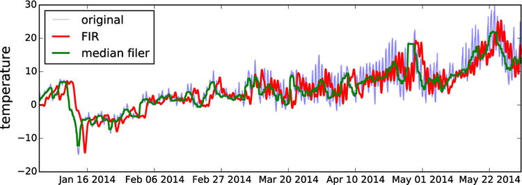
Figure 17-11. Output of an FIR filter and a median filter
The result of applying the FIR low-pass filter and the median filter to the hourly temperature measurement dataset is shown in Figure 17-11. Note that the output of the FIR filter is shifted from the original signal by a time delay that corresponds to the number of taps in the FIR filter. The median filter implemented using medfilt does not suffer from this issue because the median is computed with respect to both past and future values, which makes it a noncasual filter that cannot be evaluated on the fly on streaming input data.
In [71]: fig, ax = plt.subplots(figsize=(8, 3))
    ...: ax.plot(df.index, temperature, label="original", alpha=0.5)
    ...: ax.plot(df.index, temperature_filt, color="red", lw=2, label="FIR")
    ...: ax.plot(df.index, temperature_median_filt, color="green", lw=2, label="median filer")
    ...: ax.set_ylabel("temperature", fontsize=14)
    ...: ax.legend(loc=0)
To design an IIR filter we can use the iirdesign function from the signal module, or use one of the many predefined IIR filter types, including the Butterworth filter (signal.butter), Chebyshev filters of type I and II (signal.cheby1 and signal.cheby2), and elliptic filter (signal.ellip). For example, to create a Butterworth high-pass filter that allows frequencies above the critical frequency 7/365 to pass, while lower frequencies are suppressed, we can use:
In [72]: b, a = signal.butter(2, 7/365.0, btype='high')
The first argument to this function is the order of the Butterworth filter, and the second argument is the critical frequency of the filter (where it goes from band stop to band pass function). The optional argument btype can for example be used to specify if the filter is a low-pass filter (low) or high-pass filter (high). More options are described in the function’s docstring: See, for example, help(signal.butter). The output a and b are the ak and bk coefficients that define the IIR filter, respectively. Here we have compute a Butterworth filter of second order, so a and b each have three elements:
In [73]: b
Out[73]: array([ 0.95829139, -1.91658277,  0.95829139])
In [74]: a
Out[74]: array([ 1.        , -1.91484241,  0.91832314])
Like before we can apply the filter to an input signal (here we again use the hourly temperature dataset as an example):
In [75]: temperature_iir = signal.lfilter(b, a, temperature)
Alternatively we can apply the filter using the filtfilt function, which applies the filter both forward and backwards, resulting in a noncasual filter.
In [76]: temperature_filtfilt = signal.filtfilt(b, a, temperature)
The results of both types of filters are shown in Figure 17-12. Eliminating the low-frequency components detrends the time series and only retains the high-frequency oscillations and fluctuations. The filtered signal can therefore be viewed as measuring the volatility of the original signal. In this example we can see that the daily variations are greater during the spring months of March, April, and May, when compared to the winter months of January and February.
In [77]: fig, ax = plt.subplots(figsize=(8, 3))
    ...: ax.plot(df.index, temperature, label="original", alpha=0.5)
    ...: ax.plot(df.index, temperature_iir, color="red", label="IIR filter")
    ...: ax.plot(df.index, temperature_filtfilt, color="green", label="filtfilt filtered")
    ...: ax.set_ylabel("temperature", fontsize=14)
    ...: ax.legend(loc=0)

Figure 17-12. Output from an IIR high-pass filter and the corresponding filtfilt filter (applied both forward and backwards)
The same techniques as used above can be directly applied to the audio and image data. For example, to apply a filter to the audio signal of the guitar samples, we can use the use the lfilter functions. The coefficients bk for the FIR filter can sometimes be constructed manual. For example, to apply a naive echo sound effect, we can create a FIR filter that repeats past signals with some time delay: ![]() , where N is a time delay in units of time steps. The corresponding coefficients bk are easily constructed and can be applied to the audio signal data.
, where N is a time delay in units of time steps. The corresponding coefficients bk are easily constructed and can be applied to the audio signal data.
In [78]: b = np.zeros(10000)
    ...: b[0] = b[-1] = 1
    ...: b /= b.sum()
In [79]: data_filt = signal.lfilter(b, 1, data)
To be able to listen to the modified audio signal we can write it to a WAV file using the write function from the io.wavefile module in SciPy:
In [80]: io.wavfile.write("guitar-echo.wav", sample_rate,
    ...:                  np.vstack([data_filt, data_filt]).T.astype(np.int16))
Similarly, we can implement many types of image processing filters using the tools form the signal module. SciPy also provides a module ndimage, which contains many common image manipulation functions and filters that are especially adopted for applying on two-dimensional image data. The Scikit-Image library5 provides a more advanced framework for working with image processing in Python.
Summary
Signal processing is an extremely broad field with applications in most fields of science and engineering. As such, here we have only been able to cover a few basic applications of signal processing in this chapter, and we have focused on introducing methods for approaching this type of problem with computational methods using Python and the libraries and tools that are available within the Python ecosystem for scientific computing. In particular, we explored spectral analysis of time-dependent signals using Fast Fourier transforms, and the design and application of linear filters to signals using the signal module in the SciPy library.
Further Reading
For a comprehensive review of the theory of signal processing, see the book by Smith,, which can also be viewed online at http://www.dspguide.com/pdfbook.htm. For a Python-oriented discussion of signal processing, see the Unpingco book, from which content is available as IPython notebooks at http://nbviewer.ipython.org/github/unpingco/Python-for-Signal-Processing.
References
Smith, S. (1999). The Scientist and Engineer’s Guide to Digital Signal Processing. San Diego: Steven W. Smith.
Unpingco, J. (2014). Python for Signal Processing. New York: Springer.
________________
1There are several alternative definitions of the Fourier transform, which vary in the coefficient in the exponent and the normalization of the transform integral.
2There is also an implementation of FFT in the fft module in NumPy. It provides mostly the same functions as scipy.fftpack, which we use here. As a general rule, when SciPy and NumPy provide the same functionality, it is generally preferable to use SciPy if available, and fall back to the NumPy implementation when SciPy is not available.
3Several other window functions are also available. See the docstring for the scipy.signal module for a complete list.
4The data used in this example was obtained from https://www.freesound.org/people/guitarguy1985/sounds/52047.
5See the project’s web page at http://scikit-image.org for more information.