![]()
Statistical Modeling
In the previous chapter we covered basic statistical concepts and methods. In this chapter we build on the foundation laid out in the previous chapter and explore statistical modeling, which deals with creating models that attempt to explain data. A model can have one or several parameters, and we can use a fitting procedure to find the values of the parameter that best explains the observed data. Once a model has been fitted to data, it can be used to predict the values of new observations, given the values of the independent variables of the model. We can also perform statistical analysis on the data and the fitted model, and try to answer questions such as if the model accurately explains the data, which factors in the model is more relevant (predictive) than others, and if there are parameters that do not contribute significantly to the predictive power of the model.
In this chapter we mainly use the statsmodels library. It provides classes and functions for defining statistical models and fitting them to observed data, for calculating descriptive statistics and carrying out statistical tests. The statsmodels library has some overlap with the SciPy stats module that we covered in the previous chapter, but it is mostly an extension of what is available in SciPy.1 In particular, the main focus of the statsmodels library is on fitting models to data rather than probability distributions and random variables, for which in many cases it relies on the SciPy stats.
![]() Statsmodels The statsmodels library provides a rich set of functionality related to statistical tests and statistical modeling, including linear regression, logistic regression, and time-series analysis. For more information about the project and its documentation, see the projects web page at http://statsmodels.sourceforge.net. At the time of writing the latest version of statsmodels is 0.6.1.
Statsmodels The statsmodels library provides a rich set of functionality related to statistical tests and statistical modeling, including linear regression, logistic regression, and time-series analysis. For more information about the project and its documentation, see the projects web page at http://statsmodels.sourceforge.net. At the time of writing the latest version of statsmodels is 0.6.1.
The statsmodels library is closely integrated with the Patsy library, which allows us to write statistical models as simple formulas. The patsy library is one of the dependencies of the statsmodels library, but can also be used with other statistical libraries as well, such as for example scikit-learn that will be discussed in Chapter 15. However, here we will introduce the Patsy library in the context of using it together with the statsmodels library.
![]() Patsy The patsy library provides features for defining statistical models with a simple formula language inspired by statistical software such as R. The patsy library is designed to be a companion library for statistical modeling packages, such as statsmodels. For more information about the project and its documentation, see the web page http://patsy.readthedocs.org. At the time of writing the most recent version of patsy is 0.4.0.
Patsy The patsy library provides features for defining statistical models with a simple formula language inspired by statistical software such as R. The patsy library is designed to be a companion library for statistical modeling packages, such as statsmodels. For more information about the project and its documentation, see the web page http://patsy.readthedocs.org. At the time of writing the most recent version of patsy is 0.4.0.
Importing Modules
In this chapter we work extensively with the statsmodels library. This library encourages an import convention that is slightly different than other libraries we have used so far: it provides api modules that collect the publicly accessible symbols that the library provides. Here we assume that the statsmodels.api is imported under the name sm, and statsmodels.formula.api is imported as the name smf. We also require the statsmodels.graphics.api module to be imported as the name smg:
In [1]: import statsmodels.api as sm
In [2]: import statsmodels.formula.api as smf
In [3]: import statsmodels.graphics.api as smg
Since the statsmodels library internally uses the Patsy library, it is typically not necessary to access this library’s functions directly. However, here we directly use Patsy for demonstration purposes, and we therefore need to import the library explicitly:
In [4]: import patsy
As usual, we also require the Matplotlib, NumPy and pandas libraries to be imported as:
In [5]: import matplotlib.pyplot as plt
In [6]: import numpy as np
In [7]: import pandas as pd
and the SciPy stats module as:
In [8]: from scipy import stats
Introduction to Statistical Modeling
In this chapter we consider the following type of problem: for a set of response (dependent) variables Y, and explanatory (independent) variables X, we wish to find a mathematical relationship (model) between Y and X. In general we can write a mathematical model as a function Y = f (X ). Knowing the function f (X ) would allow us to compute the value of Y for any of values X. If we do not know the function f (X ), but we have access to data for observations {yi, xi}, we can parameterize the function f (X ) and fit the values of the parameters to the data. An example of a parameterization of f (X) is the linear model ![]() , where the coefficients β0 and β1 are the parameters of the model. Typically we have many more data points than the number of free parameters in the model. In such cases we can for example use a least-square fit that minimizes the norm of the residual
, where the coefficients β0 and β1 are the parameters of the model. Typically we have many more data points than the number of free parameters in the model. In such cases we can for example use a least-square fit that minimizes the norm of the residual ![]() , although other minimization objective functions can also be used,2 for example, depending on the statistical properties of the residual r. So far we have described a mathematical model. The essential component that makes a model statistical is that the data {yi, xi} has an element of uncertainty, for example due to measurement noise or other uncontrolled circumstances. The uncertainty in the data can be described in the model as random variables: for example,
, although other minimization objective functions can also be used,2 for example, depending on the statistical properties of the residual r. So far we have described a mathematical model. The essential component that makes a model statistical is that the data {yi, xi} has an element of uncertainty, for example due to measurement noise or other uncontrolled circumstances. The uncertainty in the data can be described in the model as random variables: for example, ![]() , where ε is a random variable. This is a statistical model because it includes random variables. Depending on how the random variables appear in the model and what distributions the random variables follow, we obtain different types of statistical models, which each may require different approaches to analyze and solve.
, where ε is a random variable. This is a statistical model because it includes random variables. Depending on how the random variables appear in the model and what distributions the random variables follow, we obtain different types of statistical models, which each may require different approaches to analyze and solve.
A typical situation where a statistical model can be useful is to describe the observations yi in an experiment, where xi is a vector with control knobs that are recorded together with each observation. An element in xi may or may not be relevant for predicting the observed outcome yi, and an important aspect of statistical modeling is to determine which explanatory variables are relevant. It is of course also possible that there are relevant factors that are not included in the set of explanatory variables xi, but which influence the outcome of the observation yi. In this case it might not be possible to accurately explain the data with the model. Determining if a model accurately explains the data is another essential aspect of statistical modeling.
A widely used statistical model is ![]() , where β0 and β1 are model parameters and ε is normally distributed with zero mean and variance s2:
, where β0 and β1 are model parameters and ε is normally distributed with zero mean and variance s2: ![]() This model is known as simple linear regression if X is a scalar, multiple linear regression if X is a vector, and if Y is a vector it is known as multivariate linear regression. Because the residual ε is normally distributed, for all these cases the model can be fitted to data using ordinary least squares (OLS). Relaxing the condition that the elements in Y, in the case of multivariate linear regression, must be independent and normally distributed with equal variance give rise to variations of the model that can be solved with methods known as generalized least squares (GLS) and weighted least squares (WLS). All methods for solving statistical models typically have a set of assumptions that one has to be mindful of when applying the models. For standard linear regression, the most important assumption is that the residuals are independent and normally distributed.
This model is known as simple linear regression if X is a scalar, multiple linear regression if X is a vector, and if Y is a vector it is known as multivariate linear regression. Because the residual ε is normally distributed, for all these cases the model can be fitted to data using ordinary least squares (OLS). Relaxing the condition that the elements in Y, in the case of multivariate linear regression, must be independent and normally distributed with equal variance give rise to variations of the model that can be solved with methods known as generalized least squares (GLS) and weighted least squares (WLS). All methods for solving statistical models typically have a set of assumptions that one has to be mindful of when applying the models. For standard linear regression, the most important assumption is that the residuals are independent and normally distributed.
The generalized linear model is an extension of the linear regression model that allows the errors in the response variable to have distributions other than the normal distribution. In particular, the response variable is assumed to be a function of a linear predictor, and where the variance of the response variable can be a function of the variable’s value. This provides a broad generalization of the linear model that is applicable in many situations. For example, this enables modeling important types of problems where the response variable takes discrete values, such as binary outcomes of count values. The errors in the response variables of such models may follow different statistical distributions (for example, the Binomial and or the Poisson distribution). Examples of these types of models include logistic regression for binary outcomes and Poisson regression for positive integer outcomes.
In the following sections we will explore how statistical models of these types can be defined and solved using the Patsy and statsmodels libraries.
Defining Statistical Models with Patsy
Common to all statistical modeling is that we need to make assumptions about the mathematical relation between the response variables Y and explanatory variables X. In the vast majority of cases we are interested in linear models, such that Y can be written as a linear combination of the response variables X, or functions of the response variables, or models that have a linear component. For example, ![]() , and
, and ![]() , and
, and ![]() , are all examples of such linear models. Note that for the model to be linear, we only need the relation to be linear with respect to the unknown coefficients α, and not necessarily in the known explanatory variables X. In contrast, an example of a nonlinear model is
, are all examples of such linear models. Note that for the model to be linear, we only need the relation to be linear with respect to the unknown coefficients α, and not necessarily in the known explanatory variables X. In contrast, an example of a nonlinear model is ![]() , since in this case Y is not a linear function with respect to β0 and β1. However, this model is log-linear in the sense that taking the logarithm of the relation yields a linear model:
, since in this case Y is not a linear function with respect to β0 and β1. However, this model is log-linear in the sense that taking the logarithm of the relation yields a linear model: ![]() for
for ![]() . Problems that can be transformed into linear model in this manner are the type of problems that can be handled with the generalized linear model.
. Problems that can be transformed into linear model in this manner are the type of problems that can be handled with the generalized linear model.
Once the mathematical form of the model has been established, the next step is typically to construct the so-called design matrices y and X such that the regression problem can be written on matrix form as ![]() , where y is the vector (or matrix) of observations, β is a vector of coefficients, and ε is the residual (error). The elements Xij of the design matrix X are the values of the (functions of) explanatory variables corresponding to each coefficient βj and observation yi. Many solvers for statistical models in statsmodels and other statistical modeling libraries can take the design matrices X and y as input.
, where y is the vector (or matrix) of observations, β is a vector of coefficients, and ε is the residual (error). The elements Xij of the design matrix X are the values of the (functions of) explanatory variables corresponding to each coefficient βj and observation yi. Many solvers for statistical models in statsmodels and other statistical modeling libraries can take the design matrices X and y as input.
For example, if the observed values are ![]() with two independent variables with corresponding values
with two independent variables with corresponding values ![]() and
and ![]() , and if the linear model under consideration is
, and if the linear model under consideration is ![]() , then the design matrix for the right-hand side is
, then the design matrix for the right-hand side is ![]() . We can construct this design matrix using the NumPy vstack function:
. We can construct this design matrix using the NumPy vstack function:
In [9]: y = np.array([1, 2, 3, 4, 5])
In [10]: x1 = np.array([6, 7, 8, 9, 10])
In [11]: x2 = np.array([11, 12, 13, 14, 15])
In [12]: X = np.vstack([np.ones(5), x1, x2, x1*x2]).T
In [13]: X
Out[13]: array([[   1.,    6.,   11.,   66.],
                [   1.,    7.,   12.,   84.],
                [   1.,    8.,   13.,  104.],
                [   1.,    9.,   14.,  126.],
                [   1.,   10.,   15.,  150.]])
Given the design matrix X and observation vector y, we can solve for the unknown coefficient vector β, for example, using least-square fit (see Chapters 5 and 6):
In [14]: beta, res, rank, sval = np.linalg.lstsq(X, y)
In [15]: beta
Out[15]: array([ -5.55555556e-01, 1.88888889e+00, -8.88888889e-01, -1.33226763e-15])
These steps are the essence of statistical modeling in its simplest form. However, variations and extensions to this basic method make statistical modeling a field in its own right, and necessitates computational frameworks such as statsmodels for systematic analysis. For example, although constructing the design matrix X was straightforward in this simple example, it can be tedious for more involved models, and if we wish to be able to easily change how the model is defined. This is where the Patsy library enters the picture. It offers a convenient (although not necessarily intuitive) formula language for defining a model and automatically constructing the relevant design matrices. To construct the design matrix for a Patsy formula we can use the patsy.dmatrices function. It takes the formula as a string as a first argument, and a dictionary-like object with data arrays for the response and explanatory variables as second arguments. The basic syntax for the Patsy formula is "y ~ x1 + x2 + ...", which means that y is a linear combination of the explanatory variables x1 and x2 (explicitly including an intercept coefficient). For a summary of the Patsy formula syntax, see Table 14-1.
Table 14-1. Simplified summary of the Patsy fomula syntax. For a complete specification of the formula syntax, see the Patsy documentation at http://patsy.readthedocs.org/en/latest
|
Syntax |
Example |
Description |
|---|---|---|
|
lhs ~ rhs |
y ~ x (Equivalent to y ~ 1 + x) |
The ~ character is used to separate the left-hand side (containing the dependent variables) and the right-hand side (containing the independent variables) of a model equation. |
|
var * var |
x1*x2 (Equivalent to x1+x2+x1*x2) |
An interaction term that implicitly contains all its lower-order interaction terms. |
|
var + var + ... |
x1 + x2 + ... (Equivalent to y ~ 1 + x1 + x2) |
The addition sign is used to denote the union of terms. |
|
var:var |
x1:x2 |
The colon character denotes a pure interaction term (for example, |
|
f(expr) |
np.log(x), np.cos(x+y) |
Arbitrary Python functions (often NumPy functions) can be used to transform terms in the expression. The expression for the argument of a function is interpreted as an arithmetic expression rather than the set-like formula operations that are otherwise used in Patsy. |
|
I(expr) |
I(x+y) |
I is a Patsy-supplied identity function that can be used to escape arithmetic expression so that they are interpreted as arithmetic operations. |
|
C(var) |
C(x), C(x, Poly) |
Treat the variable x as a categorical variable, and expand its values into orthogonal dummy variables. |
As an introductory example, consider again the linear model ![]() that we used earlier. To define this model with Patsy, we can use the formula "y ~ 1 + x1 + x2 + x1*x2". Note that we leave out coefficients in the model formula, as it is implicitly assumed that each term in the formula has a model parameter as coefficient. In addition to specifying the formula, we also need to create a dictionary data that maps the variable names to the corresponding data arrays:
that we used earlier. To define this model with Patsy, we can use the formula "y ~ 1 + x1 + x2 + x1*x2". Note that we leave out coefficients in the model formula, as it is implicitly assumed that each term in the formula has a model parameter as coefficient. In addition to specifying the formula, we also need to create a dictionary data that maps the variable names to the corresponding data arrays:
In [16]: data = {"y": y, "x1": x1, "x2": x2}
In [17]: y, X = patsy.dmatrices("y ~ 1 + x1 + x2 + x1*x2", data)
The result is two arrays y and X, which are the design matrices for the given data arrays and the specified model formula:
In [18]: y
Out[18]: DesignMatrix with shape (5, 1)
           y
           1
           2
           3
           4
           5
         Terms:
           'y' (column 0)
In [19]: X
Out[19]: DesignMatrix with shape (5, 4)
           Intercept  x1  x2  x1:x2
                   1   6  11     66
                   1   7  12     84
                   1   8  13    106
                   1   9  14    126
                   1  10  15    150
           Terms:
             'Intercept' (column 0)
             'x1' (column 1)
             'x2' (column 2)
             'x1:x2' (column 3)
These arrays are of type DesignMatrix, which is a Patsy-supplied subclass of the standard NumPy array, which contains additional metadata and an altered printing representation.
In [20]: type(X)
Out[20]: patsy.design_info.DesignMatrix
Note also that the numerical values of the DesignMatrix arrays coincide with the explicitly constructed array that we produced earlier using vstack.
As a subclass of the NumPy ndarray, the arrays of type DesignMatrix are fully compatible with code that expects NumPy arrays as input. However, we can also explicitly cast a DesignMatrix instance into an ndarray object using the np.array function, although this normally should not be necessary.
In [21]: np.array(X)
Out[21]: array([[   1.,    6.,   11.,   66.],
                [   1.,    7.,   12.,   84.],
                [   1.,    8.,   13.,  104.],
                [   1.,    9.,   14.,  126.],
                [   1.,   10.,   15.,  150.]])
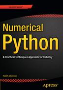
Alternatively, we can set the return_type argument to "dataframe", in which case the patsy.dmatrices function returns design matrices in the form of Pandas DataFrame objects. Also note that since DataFrame objects behave as dictionary-like objects, so we can use data frames to specify the model data as second argument to the patsy.dmatrices function.
With the help of Patsy we have now automatically created the design matrices required for solving a statistical model, using for example the np.linalg.lstsq function (as we saw an example of earlier), or using one of the many statistical-model solvers provided by the statsmodels library. For example, to perform an ordinary linear regression (OLS) we can use the class OLS from the statsmodels library instead of using the lower-level method np.linalg.lstsq. Nearly all classes for statistical models in statsmodels take the design matrices y and X and first and second argument, and returns a class instance that represents the model. To actually fit the model to the data encoded in the design matrices we need to invoke the fit method, which returns a result object that contains fitted parameters (among other attributes):
In [25]: model = sm.OLS(y, X)
In [26]: result = model.fit()
In [27]: result.params
Out[27]: Intercept   -5.555556e-01
         x1           1.888889e+00
         x2          -8.888889e-01
         x1:x2       -8.881784e-16
         dtype: float64
Note that the result is equivalent to the least-square fitting that we computed earlier in this chapter. Using the statsmodels formula API (the module that we imported as smf), we can directly pass the Patsy formula for the model when we create a model instance, which completely eliminates the need for first creating the design matrices. Instead of passing y and X as arguments, we then pass the Patsy formula and the dictionary-like object (for example, a Pandas data frame) that contains the model data.
In [28]: model = smf.ols("y ~ 1 + x1 + x2 + x1:x2", df_data)
In [29]: result = model.fit()
In [30]: result.params
Out[30]: Intercept   -5.555556e-01
         x1           1.888889e+00
         x2          -8.888889e-01
         x1:x2       -8.881784e-16
         dtype: float64
The advantage of using statsmodels instead of explicitly constructing NumPy arrays and calling the NumPy least-square model is of course that much of the processes is automated in statsmodels, which makes it possible to add and remove terms in the statistical model without any extra work. Also, when using statsmodels we have access to a large variety of linear model solvers and statistical tests for analyzing how well the model fits the data. For a summary of the Patsy formula language, see Table 14-1.
Now that we have seen how a Patsy formula can be used to construct design matrices, or be used directly with one of the many statistical model classes from statsmodels, we briefly return to the syntax and notational conventions for Patsy formulas before we continue and look in more detail on different statistical models that are available in the statsmodels library. As already mentioned above, and summarized in Table 14-1, the basic syntax for a model formula has the form “LHS ~ RHS.” The ~ character is used to separate the left-hand side (LHS) the right-hand side (RHS) of the model equation. The LHS specifies the terms that constitute the response variables, and the RHS specifies the terms that constitute the explanatory variables. The terms in the LHS and RHS expressions are separated by + or – signs, but these should not be interpreted as arithmetic operators, but rather as set union and difference operators. For example, a+b means that both a and b are included in the model, and -a means that the term a is not included in the model. An expression of the type a*b is automatically expanded to a + b + a:b, where a:b is the pure interaction term ![]() .
.
As concrete examples, consider the following formula and the resulting right-hand side terms (which we can extract from the design_info attribute using the term_names attribute):
In [31]: from collections import defaultdict
In [32]: data = defaultdict(lambda: np.array([]))
In [33]: patsy.dmatrices("y ~ a", data=data)[1].design_info.term_names
Out[33]: ['Intercept', 'a']
Here the two terms are Intercept and a, which corresponds to constant and a linear dependence on a. By default Patsy always includes the intercept constant, which in the Patsy formula also can be written explicitly using y ~ 1 + a. Including the 1 in the Patsy formula is optional.
In [34]: patsy.dmatrices("y ~ 1 + a + b", data=data)[1].design_info.term_names
Out[34]: ['Intercept', 'a', 'b']
In this case we have one more explanatory variable (a and b), and here the intercept is explicitly included in the formula. If we do not want to include the intercept in the model, we can use the notation -1 to remove this term:
In [35]: patsy.dmatrices("y ~ -1 + a + b", data=data)[1].design_info.term_names
Out[35]: ['a', 'b']
Expressions of the type a * b are automatically expanded to include all lower-order interaction terms:
In [36]: patsy.dmatrices("y ~ a * b", data=data)[1].design_info.term_names
Out[36]: ['Intercept', 'a', 'b', 'a:b']
Higher-order expansions work too:
In [37]: patsy.dmatrices("y ~ a * b * c", data=data)[1].design_info.term_names
Out[37]: ['Intercept', 'a', 'b', 'a:b', 'c', 'a:c', 'b:c', 'a:b:c']
To remove a specific term from a formula we can write the term preceded by the minus operator. For example, to remove the pure third-order interaction term a:b:c from the automatic expansion of a*b*c, we can use:
In [38]: patsy.dmatrices("y ~ a * b * c - a:b:c", data=data)[1].design_info.term_names
Out[38]: ['Intercept', 'a', 'b', 'a:b', 'c', 'a:c', 'b:c']
In Patsy, the + and - operators are used for set-like operations on sets of terms, if we need to represent the arithmetic operations we need to wrap the expression in a function call. For convenience, Patsy provides an identity function with the name I that can be used for this purpose. To illustrate this point, consider the following two examples, which show the resulting terms for y ~ a + b and y ~ I(a + b):
In [39]: data = {k: np.array([]) for k in ["y", "a", "b", "c"]}
In [40]: patsy.dmatrices("y ~ a + b", data=data)[1].design_info.term_names
Out[40]: ['Intercept', 'a', 'b']
In [41]: patsy.dmatrices("y ~ I(a + b)", data=data)[1].design_info.term_names
Out[41]: ['Intercept', 'I(a + b)']
Here the column in the design matrix that corresponds to the term with the name I(a+b) is the arithmetic sum of the arrays for the variables a and b. The same trick must be used if we want to include terms that are expressed as a power of a variable:
In [42]: patsy.dmatrices("y ~ a**2", data=data)[1].design_info.term_names
Out[42]: ['Intercept', 'a']
In [43]: patsy.dmatrices("y ~ I(a**2)", data=data)[1].design_info.term_names
Out[43]: ['Intercept', 'I(a ** 2)']
The notation I(...) that we used here is an example of a function call notation. We can apply transformations of the input data in a Patsy formula by including arbitrary Python function calls in the formula. In particular, we can transform the input data array using functions from NumPy:
In [44]: patsy.dmatrices("y ~ np.log(a) + b", data=data)[1].design_info.term_names
Out[44]: ['Intercept', 'np.log(a)', 'b']
Or we can even transform variables with arbitrary Python functions:
In [45]: z = lambda x1, x2: x1+x2
In [46]: patsy.dmatrices("y ~ z(a, b)", data=data)[1].design_info.term_names
Out[46]: ['Intercept', 'z(a, b)']
So far we have considered models with numerical response and explanatory variables. Statistical modeling also frequently includes categorical variables, which can take a discrete set of values that do not have meaningful numerical order (for example, “Female” or “Male” type “A,” “B,” or “C,” etc.). When using such variables in a linear model we typically need to recode them by introducing binary dummy variables. In a patsy formula any variable that does not have a numerical data type (float or int) will be interpreted as a categorical variable, and automatically encoded accordingly. For numerical variable we can use the C(x) notation to explicitly request that a variable x should be treated as a categorical variable.
For example, compare the following two examples that show the design matrix for the formula "y ~ - 1 + a" and "y ~ - 1 + C(a)", which corresponds to models where a is a numerical and categorical explanatory variable, respectively:

For a numerical variable the corresponding column in the design matrix simply corresponds to the data vector, while for a categorical variable C(a) new binary-valued columns with a mask-like encoding of individual values of the original variable:

Variables with non-numerical values are automatically interpreted and treated as categorical values:

The default type of encoding of categorical variables into binary-valued treatment fields can be changed and extended by the user. For example, to encode the categorical variables with orthogonal polynomials instead of treatment indicators, we can use C(a, Poly):

The automatic encoding of categorical variables by Patsy is a very convenient aspect of Patsy formula, which allows the user to easily add a remove both numerical and categorical variables in a model. This is arguably one of the main advantages of the using the Patsy library to define model equations.
Linear Regression
The statsmodels library support several types of statistical models that are applicable in varying situations, but nearly all of them follow the same usage pattern, which makes it easy to switch between different models. Statistical models in statsmodels are represented by model classes. These can be initiated given the design matrices for the response and explanatory variables of a linear model, or given a Patsy formula and a data frame (or other dictionary-like object). The basic workflow when setting up and analyzing a statistical model with statsmodels includes the following steps:
- Create an instance of model class, for example, using model = sm.MODEL(y, X) or model = smf.model(formula, data), where MODEL and model are the names of a particular model, such as OLS, GLS, Logit, etc. Here the convention is that uppercase names are used for classes that takes design matrices as arguments, and lowercase names for classes that takes Patsy formulas and data frames as arguments.
- Creating a model instance does not perform any computations. To fit the model to the data we must invoke the fit method, result = model.fit(), which performs the fit and returns a result object that have methods and attributes for further analysis.
- Print summary statistics for the result object returned by the fit method. The result object varies in content slightly for each statistical model, but most models implement the method summary, which produces a summary text that describes the result of the fit, including several types of statistics that can be useful for judging if the statistical model successfully explains the data. Viewing the output from the summary method is usually a good starting pointing when analyzing the result of a fitting process.
- Post-process the model fit results: in addition to the summary method, the result object also contains methods and attributes for obtaining the fitted parameters (params), the residual for the model and the data (resid), the fitted values (fittedvalues), and a method for predicting the value of the response variables for new independent variables (predict).
- Finally it may be useful to visualize the result of the fitting, for example, with the Matplotlib and Seaborn graphics libraries, or using some of the many graphing routines that are directly included in the statsmodels library (see the statsmodels.graphics module).
To demonstrate this workflow with a simple example, in the following we consider fitting a model to generated data whose true value is ![]() . We begin with storing the data in a Pandas data frame object:
. We begin with storing the data in a Pandas data frame object:
In [53]: N = 100
In [54]: x1 = np.random.randn(N)
In [55]: x2 = np.random.randn(N)
In [56]: data = pd.DataFrame({"x1": x1, "x2": x2})
In [57]: data["y_true"] = 1  + 2 * x1 + 3 * x2 + 4 * x1 * x2
Here we have stored the true value of y in the y_true column in the DataFrame object data. We simulate a noisy observation of y by adding a normal-distributed noise to the true values, and store the result in the y column:
In [58]: e = 0.5 * np.random.randn(N)
In [59]: data["y"] = data["y_true"] + e
Now, from the data we know that we have two explanatory variables, x1 and x2, in addition to the response variable y. The simplest possible model we can start with is the linear model ![]() , which we can define with the Patsy formula "y ~ x1 + x2". Since the response variable is continuous, it is a good starting point to fit the model to the data using ordinary linear square, for which we can use the smf.ols class.
, which we can define with the Patsy formula "y ~ x1 + x2". Since the response variable is continuous, it is a good starting point to fit the model to the data using ordinary linear square, for which we can use the smf.ols class.
In [60]: model = smf.ols("y ~ x1 + x2", data)
In [61]: result = model.fit()
Remember that ordinary least-square regression assumes that the residuals of the fitted model and the data is normally distributed. However, before analyzing the data we might not know if this condition is satisfied or not. Nonetheless, we can start with fitting the data to the model and investigate the distribution of the residual using graphical methods and statistical tests (with null hypothesis that the residuals are indeed normally distributed). A lot of useful information, including several types of test statistics, can be display using the summary method:
In [62]: print(result.summary())
                            OLS Regression Results
==============================================================================
Dep. Variable:                      y   R-squared:                       0.380
Model:                            OLS   Adj. R-squared:                  0.367
Method:                 Least Squares   F-statistic:                     29.76
Date:                Wed, 22 Apr 2015   Prob (F-statistic):           8.36e-11
Time:                        22:40:33   Log-Likelihood:                -271.52
No. Observations:                 100   AIC:                             549.0
Df Residuals:                      97   BIC:                             556.9
Df Model:                           2
Covariance Type:            nonrobust
==============================================================================
                 coef    std err          t      P>|t|      [95.0% Conf. Int.]
------------------------------------------------------------------------------
Intercept      0.9868      0.382      2.581      0.011         0.228     1.746
x1             1.0810      0.391      2.766      0.007         0.305     1.857
x2             3.0793      0.432      7.134      0.000         2.223     3.936
==============================================================================
Omnibus:                       19.951   Durbin-Watson:                   1.682
Prob(Omnibus):                  0.000   Jarque-Bera (JB):               49.964
Skew:                          -0.660   Prob(JB):                     1.41e-11
Kurtosis:                       6.201   Cond. No.                         1.32
==============================================================================
Warnings: [1] Standard Errors assume that the covariance matrix of the errors is correctly specified.
The output produced by the summary method is rather verbose, and a detailed description of all the information provided by this method is beyond the scope of this treatment. Instead, here we only focus on a few key indicators. To begin with, the R-squared value is a statistic that indicates of how well the model fits the data. It can take values between 0 and 1, where an R-squared statistic of 1 corresponds to a perfect fit. The R-squared value of 0.380 reported above is rather poor, and it indicates that we need to refine our model (which is expected, since we left out the interaction term ![]() ). We can also explicitly access the R-squared statistic from the result object using the rsquared attribute.
). We can also explicitly access the R-squared statistic from the result object using the rsquared attribute.
In [63]: result.rsquared
Out[63]: 0.38025383255132539
Furthermore, the coef column in the middle of the table provides the fitted model parameters. Assuming that the residuals indeed are normally distributed, the std err column provides an estimate of the standard errors for the model coefficients, and the t and P>|t| columns are the t-statistics and the corresponding p-value for the statistical test with the null hypothesis that the corresponding coefficient is zero. Therefore, while keeping in mind that this analysis assumes that the residuals are normally distributed, we can look for the columns with small p-values and judge which explanatory variables have coefficients that are very likely to be different from zero (meaning that they have a significant predictive power).
To investigate whether the assumption of normal-distributed errors is justified we need to look at the residuals of the model fit to the data. The residuals are accessible via the resid attribute of the result object:
In [64]: result.resid.head()
Out[64]: 0    -3.370455
         1    -11.153477
         2    -11.721319
         3    -0.948410
         4    0.306215
         dtype: float64
Using these residuals, we can check for normality using the normaltest function from the SciPy stats module:
In [65]: z, p = stats.normaltest(result.fittedvalues.values)
In [66]: p
Out[66]: 4.6524990253009316e-05
For this example the resulting p-value is indeed very small, suggesting that we can reject the null hypothesis that the residuals are normally distributed (that is, we can conclude that the assumption of normal-distributed residuals is violated). A graphical method to check for normality of a sample is to use the qqplot from the statsmodels.graphics module. The QQ-plot, which compares the sample quantiles with the theoretical quantiles, should be close to a straight line if the sampled values are indeed normally distributed. The following function call to smg.qqplot produces the QQ-plot shown in Figure 14-1:
In [67]: fig, ax = plt.subplots(figsize=(8, 4))
    ...: smg.qqplot(result.resid, ax=ax)

Figure 14-1. QQ-plot of a linear model with two explanatory variables without interaction term
As can be seen in Figure 14-1, the points in the QQ-plot significantly deviate for a linear relation, suggesting that the observed residuals are unlikely to be a sample of a normal-distributed random variable. In summary, these indicators provide evidence that the model that we use is not sufficient, and that we might need to refine the model. We can include the missing interaction term by adding it to the Patsy formula and repeat the steps from the previous analysis:
In [68]: model = smf.ols("y ~ x1 + x2 + x1*x2", data)
In [69]: result = model.fit()
In [70]: print(result.summary())
                            OLS Regression Results
==============================================================================
Dep. Variable:                      y   R-squared:                       0.963
Model:                            OLS   Adj. R-squared:                  0.961
Method:                 Least Squares   F-statistic:                     821.8
Date:                Tue, 21 Apr 2015   Prob (F-statistic):           2.69e-68
Time:                        23:52:12   Log-Likelihood:                -138.39
No. Observations:                 100   AIC:                             284.8
Df Residuals:                      96   BIC:                             295.2
Df Model:                           3
Covariance Type:            nonrobust
==============================================================================
                 coef    std err          t      P>|t|      [95.0% Conf. Int.]
------------------------------------------------------------------------------
Intercept      1.1023      0.100     10.996      0.000         0.903     1.301
x1             2.0102      0.110     18.262      0.000         1.792     2.229
x2             2.9085      0.095     30.565      0.000         2.720     3.097
x1:x2          4.1715      0.134     31.066      0.000         3.905     4.438
==============================================================================
Omnibus:                        1.472   Durbin-Watson:                   1.912
Prob(Omnibus):                  0.479   Jarque-Bera (JB):                0.937
Skew:                           0.166   Prob(JB):                        0.626
Kurtosis:                       3.338   Cond. No.                         1.54
==============================================================================
Warnings: [1] Standard Errors assume that the covariance matrix of the errors is correctly specified.
In this case we can see that the R-squared statistic is significantly higher, 0.963, indicating a nearly perfect correspondence between the model and the data.
In [71]: result.rsquared
Out[71]: 0.96252198253140375
Note that we can always increase the R-squared statistic by introducing more variables, but we want to make sure that we do not add variables with low predictive power (small coefficient and high corresponding p-value), since it would make the model susceptible to overfitting, and as usual we require that the residuals be normally distributed. Repeating the normality test and the QQ-plot form previous analysis with the updated model results in a relatively high p-value (0.081) and a relatively linear QQ-plot (see Figure 14-2). This suggests that in this case the residuals could very well be normally distributed (as we know they are, by design, in this example).
In [72]: z, p = stats.normaltest(result.fittedvalues.values)
In [73]: p
Out[73]: 0.081352587523644201
In [74]: fig, ax = plt.subplots(figsize=(8, 4))
    ...: smg.qqplot(result.resid, ax=ax)

Figure 14-2. QQ-plot of a linear model with two explanatory variables with interaction term
Once we are satisfied with the fit of the model, we can extract the model coefficients from the result object using the params attribute.
In [75]: result.params
Out[75]: Intercept    1.102297
         x1           2.010154
         x2           2.908453
         x1:x2        4.171501
         dtype: float64
Also, we can predict the values of new observations using the predict method, which takes as argument a NumPy array or DataFrame object with values of the independent variables (x1 and x2 in this case). For example, since the current problem has only two independent variables we can visualize the predictions of the model as a contour plot. To this end we first construct a DataFrame object with the x1 and x2 values for which we want to predict the y value for using the fitted model.
In [76]: x = np.linspace(-1, 1, 50)
In [77]: X1, X2 = np.meshgrid(x, x)
In [78]: new_data = pd.DataFrame({"x1": X1.ravel(), "x2": X2.ravel()})
Using the predict method of the result object obtained from the fitting of the model we can compute the predicted y values for the new set of values of the response variables.
In [79]: y_pred = result.predict(new_data)
The result is a NumPy array (vector) with the same length as the data vectors X1.ravel() and X2.ravel(). To be able to plot the data using the Matplotlib contour function we first resize the y_pred vector to a square matrix.
In [80]: y_pred.shape
Out[80]: (2500,)
In [81]: y_pred = y_pred.reshape(50, 50)
The contour graphs of the true model and the fitted model are shown in Figure 14-3, which demonstrate that the agreement of the model fitted to the 100 noisy observations of y is sufficient to reproduce the function rather accurately in this example.
In [82]: fig, axes = plt.subplots(1, 2, figsize=(12, 5), sharey=True)
    ...: def plot_y_contour(ax, Y, title):
    ...:     c = ax.contourf(X1, X2, Y, 15, cmap=plt.cm.RdBu)
    ...:     ax.set_xlabel(r"$x_1$", fontsize=20)
    ...:     ax.set_ylabel(r"$x_2$", fontsize=20)
    ...:     ax.set_title(title)
    ...:     cb = fig.colorbar(c, ax=ax)
    ...:     cb.set_label(r"$y$", fontsize=20)
    ...:
    ...: plot_y_contour(axes[0], y_true(X1, X2), "true relation")
    ...: plot_y_contour(axes[1], y_pred, "fitted model")

Figure 14-3. The true relation and fit of the correct model to 100 sample from the true relation with normal-distributed noise
In the example we have looked at here we used the ordinary least-square (ols) method to fit the model to the data. Several other options are also available, such as the robust linear model (rlm) that is suitable if there are significant outliers in the observations, and variants of the generalized linear model that is suitable, for example, if the response variable can take only discrete values. This is the topic of the following section. In the following chapter we will also see examples of regularized regression, where the minimization criteria is modified to not only minimize the square of the residuals, but also, for example, to penalize large coefficients in the model.
Example Datasets
When working with statistical methods it is helpful to have example datasets to explore. The statsmodels package provides an interface for loading examples datasets from an extensive dataset repository3 from the R statistical software. The module sm.datasets contains a function get_rdataset that can be used to load datasets listed on the page http://vincentarelbundock.github.io/Rdatasets/datasets.html. The get_rdataset function takes the name of the dataset and optionally also the name of a package (grouping of datasets).
For example, to load a dataset named Icecream from the package Ecdat, we can use:
In [83]: dataset = sm.datasets.get_rdataset("Icecream", "Ecdat")
The result is a data structure with the dataset and metadata describing the dataset. The name of the dataset is given by the title attribute, and the __doc__ attribute contains an explanatory text describing the dataset (too long to display here):
In [84]: dataset.title
Out[84]: 'Ice Cream Consumption'
The data in the form of a Pandas DataFrame object is accessible via the data attribute:
In [85]: dataset.data.info()
<class 'pandas.core.frame.DataFrame'>
Int64Index: 30 entries, 0 to 29
Data columns (total 4 columns):
cons      30 non-null float64
income    30 non-null int64
price     30 non-null float64
temp      30 non-null int64
dtypes: float64(2), int64(2)
memory usage: 1.2 KB
From the information given by the DataFrame info method we can see that the Icecream dataset contains four variables: cons (consumption), income, price, and temp (temperature). Once a dataset is loaded we can explore it and fit it to statistical models following the usual procedures. For example, to model the consumption with as a linear model with price and temperature as independent variables, we can use:
In [86]: model = smf.ols("cons ~ -1 + price + temp", data=dataset.data)
In [87]: result = model.fit()
The result object can be analyzed using descriptive statistics and statistical tests, for example, starting with printing the output from the summary method, as we have seen before. We can also take a graphical approach and plot regression graphs, for example, using the plot_fit function in the smg module (see also the regplot function in the seaborn library):
In [88]: fig, (ax1, ax2) = plt.subplots(1, 2, figsize=(12, 4))
    ...: smg.plot_fit(result, 0, ax=ax1)
    ...: smg.plot_fit(result, 1, ax=ax2)
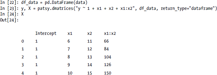
From the regression plots shown in Figure 14-4, we can conclude that in this Icecream dataset the consumption seems linearly correlated to the temperature but has no clear dependence on the price (probably because the range of prices is rather small). Graphical tools such as plot_fit can be useful tools when developing statistical models.
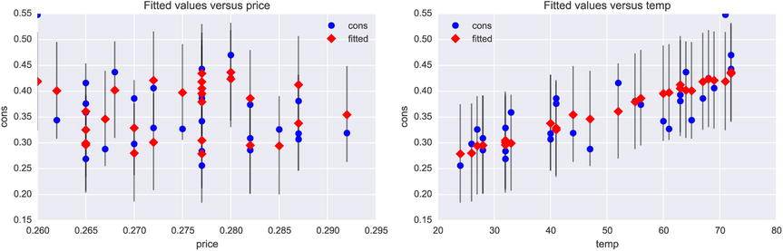
Figure 14-4. Regression plots for the fit of the consumption versus price and temperature in the Icecream dataset
Discrete Regression
Regression with discrete dependent variables (for example, binary outcomes) requires different techniques than the linear regression model that we have seen so far. The reason is that linear regression requires that the response variable is a normal-distributed continuous variable, which cannot be used directly for a response variable that has only a few discrete possible outcomes, such as binary variables or variables taking positive integer values. However, using a suitable transformation it is possible to map a linear predictor to an interval that can be interpreted as a probability of different discrete outcomes. For example, in the case of binary outcomes, one popular transformation is the logistic function ![]() , or
, or ![]() , which maps
, which maps ![]() to
to ![]() . In other words, the continuous or discrete feature vector x is mapped via the model parameters β0 and β1 and the logistic transformation onto a probability p. If
. In other words, the continuous or discrete feature vector x is mapped via the model parameters β0 and β1 and the logistic transformation onto a probability p. If ![]() , it can be taken to predict that
, it can be taken to predict that ![]() , and
, and ![]() can be taken to predict
can be taken to predict ![]() . This procedure, which is known as logistic regression, is an example of a binary classifier. We will see more about classifiers in Chapter 15 (about machine learning).
. This procedure, which is known as logistic regression, is an example of a binary classifier. We will see more about classifiers in Chapter 15 (about machine learning).
The statsmodels library provides several methods for discrete regression, including the Logit class,4 the related Probit class (which uses a cumulative distribution function of the normal distribution rather than the logistic function to transform the linear predictor to the [0, 1] interval), the multinomial logistic regression class MNLogit (for more than two categories), and the Poisson regression class Poisson for Poisson-distributed count variables (positive integers).
Logistic Regression
As an example of how to perform a logistic regression with statsmodels, we first load a classic dataset using the sm.datasets.get_rdataset function, which contains sepal and petal lengths and width for a sample of Iris flowers, together with a classification of the species of the flower. Here we will select a subset of the dataset corresponding to two different species, and create a logistic model for predicting the type of species from the values of the petal length and width. The info method gives a summary of which variables are contained in the dataset:
In [89]: df = sm.datasets.get_rdataset("iris").data
In [90]: df.info()
<class 'pandas.core.frame.DataFrame'>
Int64Index: 150 entries, 0 to 149
Data columns (total 5 columns):
Sepal.Length    150 non-null float64
Sepal.Width     150 non-null float64
Petal.Length    150 non-null float64
Petal.Width     150 non-null float64
Species         150 non-null object
dtypes: float64(4), object(1)
memory usage: 7.0+ KB
To see how many unique types of species are present in the Species column we can use the unique method for the Pandas series that is returned when extracting the column from the data frame object:
In [91]: df.Species.unique()
Out[91]: array(['setosa', 'versicolor', 'virginica'], dtype=object)
This dataset contains three different types of species. To obtain a binary variable that we can use as response variable in a logistic regression, here we focus only on the data for the two species versicolor and virginica. For convenience we create a new data frame, df_subset, for the subset of the dataset corresponding to those species:
In [92]: df_subset = df[(df.Species == "versicolor") | (df.Species == "virginica")].copy()
To be able to use logistic regression to predict the species using the other variables as independent variables, we first need to create a binary variable that corresponds to the two difference species. Using the map method of the Pandas series object we can map the two species names into binary values 0 and 1.
In [93]: df_subset.Species = df_subset.Species.map({"versicolor": 1, "virginica": 0})
We also need to rename the columns with names that contain period characters to names that are valid symbol names in Python (for example by replacing the “.” characters with “_”), or else Patsy formulas that including these column names will be interpreted incorrectly. To rename the columns in a DataFrame object we can use the rename method and by passing a dictionary with name translations as the columns argument:
In [94]: df_subset.rename(columns={"Sepal.Length": "Sepal_Length",
    ...:                           "Sepal.Width": "Sepal_Width",
    ...:                           "Petal.Length": "Petal_Length",
    ...:                           "Petal.Width": "Petal_Width"}, inplace=True)
After these transformations we have a DataFrame instance that is suitable for use in a logistic regression analysis:

To create a logistic model that attempts to explain the value of the Species variable with Petal_length and Petal_Width as independent variables, we can create an instance of the smf.logit class and using the Patsy formula "Species ~ Petal_Length + Petal_Width":
In [96]: model = smf.logit("Species ~ Petal_Length + Petal_Width", data=df_subset)
As usual, we need to call the fit method of the resulting model instance to actually fit the model to the supplied data. The fit is performed with maximum likelihood optimization.
In [97]: result = model.fit()
Optimization terminated successfully.
          Current function value: 0.102818
          Iterations 10
As for regular linear regression, we can obtain a summary of the fit of the model to the data by printing the output produced by the summary method in the result object. In particular, we can see the fitted model parameters with an estimate for its z-score and the corresponding p-value, which can help us judge whether an explanatory variable is significant or not in the model.
In [98]: print(result.summary())
                           Logit Regression Results
==============================================================================
Dep. Variable:                Species   No. Observations:                  100
Model:                          Logit   Df Residuals:                       97
Method:                           MLE   Df Model:                            2
Date:                Sun, 26 Apr 2015   Pseudo R-squ.:                  0.8517
Time:                        01:41:04   Log-Likelihood:                -10.282
converged:                       True   LL-Null:                       -69.315
LLR p-value:                 2.303e-26
================================================================================
                   coef    std err          z      P>|z|      [95.0% Conf. Int.]
--------------------------------------------------------------------------------
Intercept       45.2723     13.612      3.326      0.001        18.594    71.951
Petal_Length    -5.7545      2.306     -2.496      0.013       -10.274    -1.235
Petal_Width    -10.4467      3.756     -2.782      0.005       -17.808    -3.086
================================================================================
The result object for logistic regression also provides the method get_margeff, which returns an object that also implements a summary method that outputs information about the marginal effects of each explanatory variable in the model.
In [99]: print(result.get_margeff().summary())
        Logit Marginal Effects
=====================================
Dep. Variable:                Species
Method:                          dydx
At:                           overall
================================================================================
                  dy/dx    std err          z      P>|z|      [95.0% Conf. Int.]
--------------------------------------------------------------------------------
Petal_Length    -0.1736      0.052     -3.347      0.001        -0.275    -0.072
Petal_Width     -0.3151      0.068     -4.608      0.000        -0.449    -0.181
================================================================================
When we are satisfied with the fit of the model to the data, we can use it to predict the value of the response variable for new values of the explanatory variables. For this we can use the predict method in the result object produced by the model fitting, and to it we need to pass a data frame object with the new values of the independent variables.
In [100]: df_new = pd.DataFrame({"Petal_Length": np.random.randn(20)*0.5 + 5,
     ...:                        "Petal_Width": np.random.randn(20)*0.5 + 1.7})
In [101]: df_new["P-Species"] = result.predict(df_new)
The result is an array with probabilities for each observation to correspond to the response ![]() , and by comparing this probability to the threshold value 0.5 we can generate predictions for the binary value of the response variable:
, and by comparing this probability to the threshold value 0.5 we can generate predictions for the binary value of the response variable:
In [102]: df_new["P-Species"].head(3)
Out[102]: 0    0.995472
          1    0.799899
          2    0.000033
                Name: P-Species, dtype: float64
In [103]: df_new["Species"] = (df_new["P-Species"] > 0.5).astype(int)
The intercept and the slope of the line in the plane spanned by the coordinates Petal_Width and Petal_Length that defines the boundary between a point that is classified as ![]() and
and ![]() , respectively, can be computed from the fitted model parameters. The model parameters can be obtained using the params attribute of the result object:
, respectively, can be computed from the fitted model parameters. The model parameters can be obtained using the params attribute of the result object:
In [104]: params = result.params
     ...: alpha0 = -params['Intercept']/params['Petal_Width']
     ...: alpha1 = -params['Petal_Length']/params['Petal_Width']
Finally, to access the model and its predictions for new data points, we plot a scatter plot of the fitted (squares) and predicted (circles) data where data corresponding to the species virginica is coded with blue color, and the species versicolor is coded with green color. The result is shown in Figure 14-5.
In [105]: fig, ax = plt.subplots(1, 1, figsize=(8, 4))
     ...: # species virginica
     ...: ax.plot(df_subset[df_subset.Species == 0].Petal_Length.values,
     ...:         df_subset[df_subset.Species == 0].Petal_Width.values, 's',
     ...:         label='virginica')
     ...: ax.plot(df_new[df_new.Species == 0].Petal_Length.values,
     ...:         df_new[df_new.Species == 0].Petal_Width.values,
     ...:         'o', markersize=10, color="steelblue", label='virginica (pred.)')
     ...:
     ...: # species versicolor
     ...: ax.plot(df_subset[df_subset.Species == 1].Petal_Length.values,
     ...:         df_subset[df_subset.Species == 1].Petal_Width.values, 's',
     ...:         label='versicolor')
     ...: ax.plot(df_new[df_new.Species == 1].Petal_Length.values,
     ...:         df_new[df_new.Species == 1].Petal_Width.values,
     ...:         'o', markersize=10, color="green", label='versicolor (pred.)')
     ...:
     ...: # boundary line
     ...: _x = np.array([4.0, 6.1])
     ...: ax.plot(_x, alpha0 + alpha1 * _x, 'k')
     ...: ax.set_xlabel('Petal length')
     ...: ax.set_ylabel('Petal width')
     ...: ax.legend()
Figure 14-5. The result of a classification of Iris species using Logit regression with petal length and width and independent variables
Poisson Model
Another example of discrete regression is the Poisson model, which describes a process where the response variable is a success count for many attempts that each has a low probability of success. The Poisson model is also an example of a model that can be treated with the generalized linear model, using the natural logarithm as link function. To see how we can fit data to a Poisson model using the statsmodels library, we will analyze another interesting dataset from the R dataset repository: The discoveries dataset contains counts of the number of great discoveries between 1860 and 1959. Because of the nature of the data it reasonable to assume that the counts might be Poisson distributed. To explore this hypothesis we begin with loading the dataset using the sm.datasets.get_rdataset function and display the first few values to obtain an understanding of the format of the data.

Here we can see that the dataset contains integer counts in the discoveries series, and that the first few years in the series have, on average, a few great discoveries. To see if this is typical data for the entire series we can plot a bar graph of the number of discoveries per year, as shown in Figure 14-6.
In [109]: fig, ax = plt.subplots(1, 1, figsize=(16, 4))
     ...: df.plot(kind='bar', ax=ax)

Figure 14-6. The number of great discoveries per year
Judging from Figure 14-6, the number of great discoveries seems to be relatively constant over time, although a slight declining trend might be noticeable. Nonetheless, the initial hypothesis that the number of discoveries might be Poisson distributed does not look immediately unreasonable. To explore this hypothesis more systematically we can fit the data to a Poisson process, for example, using the smf.poisson class and the Patsy formula "discoveries ~ 1", which means that we model the discoveries variable with only an intercept coefficient (the Poisson distribution parameter).
In [110]: model = smf.poisson("discoveries ~ 1", data=df)
As usual we have to call the fit method to actually perform the fit of the model to the supplied data:
In [111]: result = model.fit()
Optimization terminated successfully.
          Current function value: 2.168457
          Iterations 7
The summary method of the result objects displays a summary of model fit and several fit statistics.
In [112]: print(result.summary())
                          Poisson Regression Results
==============================================================================
Dep. Variable:            discoveries   No. Observations:                  100
Model:                        Poisson   Df Residuals:                       99
Method:                           MLE   Df Model:                            0
Date:                Sun, 26 Apr 2015   Pseudo R-squ.:                   0.000
Time:                        14:51:41   Log-Likelihood:                -216.85
converged:                       True   LL-Null:                       -216.85
LLR p-value:                       nan
==============================================================================
                 coef    std err          z      P>|z|      [95.0% Conf. Int.]
------------------------------------------------------------------------------
Intercept      1.1314      0.057     19.920      0.000         1.020     1.243
==============================================================================
The model parameters, available via the params attribute of the result object, is related to the λ parameter of the Poisson distribution via the exponential function (the inverse of the link function):
In [113]: lmbda = np.exp(result.params)
Once we have the estimated λ parameter of the Poisson distribution we can compare the histogram of the observed counts values with the theoretical counts, which we can obtain from a Poisson-distributed random variable from the SciPy stats library.
In [114]: X = stats.poisson(lmbda)
In addition to the fit parameters we can also obtain estimated confidence intervals of the parameters using the conf_int method:

To assess the fit of the data to the Poisson distribution we also create random variables for the lower and upper bounds of the confidence interval for the model parameter:
In [116]: X_ci_l = stats.poisson(np.exp(result.conf_int().values)[0, 0])
In [117]: X_ci_u = stats.poisson(np.exp(result.conf_int().values)[0, 1])
Finally we graph the histogram of the observed counts with the theoretical probability mass functions for the Poisson distributions corresponding to the fitted model parameter and its confidence intervals. The result is shown in Figure 14-7.
In [118]: v, k = np.histogram(df.values, bins=12, range=(0, 12), normed=True)
In [119]: fig, ax = plt.subplots(1, 1, figsize=(12, 4))
     ...: ax.bar(k[:-1], v, color="steelblue",  align='center', label='Dicoveries per year')
     ...: ax.bar(k-0.125, X_ci_l.pmf(k), color="red", alpha=0.5, align='center', width=0.25,
     ...:        label='Poisson fit (CI, lower)')
     ...: ax.bar(k, X.pmf(k), color="green",  align='center', width=0.5, label='Poisson fit')
     ...: ax.bar(k+0.125, X_ci_u.pmf(k), color="red",  alpha=0.5, align='center', width=0.25,
     ...:        label='Poisson fit (CI, upper)')
     ...: ax.legend()

Figure 14-7. Comparison of histogram of the number of great discoveries per year and the probability mass function for the fitted Poisson model
The result shown in Figure 14-7 indicates that the dataset of great discoveries are not well described by a Poisson process, since the agreement between Poisson probability mass function and the observed counts deviates significantly. The hypothesis that the great discoveries per year are a Poisson process must therefore be rejected. A failure to fit a model to a given dataset is of course a natural part of statistical modeling process, and although the dataset turned out not to be Poisson distributed (perhaps because years with a large and small number of great discovers tend to be clustered together), we still have gained insight by the failed attempt to model it as such. Because of the correlations between the number of discoveries at any given year and its recent past, a time-series analysis such as discussed in the following section could be a better approach.
Time Series
Time-series analysis is an important field in statistical modeling that deals with analyzing and forecasting future values of data that is observed as a function of time. Time-series modeling differs in several aspects from the regular regression models that we have looked at so far. Perhaps most importantly, a time-series of observations typically cannot be considered as a series of independent random samples from a population. Instead there is often a rather strong component of correlation between observations that are close to each other in time. Also, the independent variables in a time-series model are the past observations of the same series, rather than a set of distinct factors. For example, while a regular regression can describe the demand for a product as a function of its price, in a time-series model it is typical to attempt to predict the future values from the past observations. This is a reasonable approach when there are autocorrelations such as trends in the time series under consideration (for example, daily or weekly cycles, or steady increasing trends, or inertia in the change of its value). Examples of time series include stock prices, weather and climate observations, and many other temporal processes in nature and in economics.
An example of a type of statistical model for time series is the autoregressive (AR) model, in which a future value depends linearly on p previous values: ![]() , where β0 is a constant and
, where β0 is a constant and ![]() , are the coefficients that define the AR model. The error εt is assumed to be white noise without autocorrelation. Within this model, all autocorrelation in the time series should therefore be captured by the linear dependence on the p previous values. A time series that depends linearly on only one previous value (in a suitable unit of time) can be fully modeled with an AR process with p =1, denoted as AR(1), and a time series that depends linearly on two previous values can be modeled by a AR(2) process, and so on. The AR model is a special case of the ARMA model, a more general model that also include a moving average (MA) of q previous residuals of the series:
, are the coefficients that define the AR model. The error εt is assumed to be white noise without autocorrelation. Within this model, all autocorrelation in the time series should therefore be captured by the linear dependence on the p previous values. A time series that depends linearly on only one previous value (in a suitable unit of time) can be fully modeled with an AR process with p =1, denoted as AR(1), and a time series that depends linearly on two previous values can be modeled by a AR(2) process, and so on. The AR model is a special case of the ARMA model, a more general model that also include a moving average (MA) of q previous residuals of the series:  , where the model parameters θn are the weight factors for the moving averaging. This model is known as the ARMA model, and is denoted ARMA(p, q), where p is the number of autoregressive terms and q is the number of moving-average terms. Many other models for time-series model exists, but the AR and ARMA capture the basic ideas that are fundamental to many time-series applications.
The statsmodels library has a submodule dedicated to time-series analysis: sm.tsa, which implements several standard models for time-series analysis, as well as graphical and statistical analysis tools for exploring properties of time-series data. For example, let’s revisit the time series with outdoors temperature measurements used in Chapter 12, and say that we want to predict the hourly temperature of for few days into the future based on previous observations using an AR model. For concreteness, we will take the temperatures measured during the month of March and predict the hourly temperature of the first three days of April. We first load the dataset into a Pandas DataFrame object:
In [120]: df = pd.read_csv("temperature_outdoor_2014.tsv", header=None, delimiter="	",
     ...:                  names=["time", "temp"])
     ...: df.time = pd.to_datetime(df.time, unit="s")
     ...: df = df.set_index("time").resample("H")
For convenience we extract the observations for March and April and store them in new DataFrame objects, df_march and df_april, respectively:
In [121]: df_march = df[df.index.month == 3]
In [122]: df_april = df[df.index.month == 4]
Here we will attempt to model the time series of the temperature observations using the AR model, and an important condition for its applicability is that it is applied to a stationary process, which does not have autocorrelation or trends other than those explained by the terms in the model. The function plot_acf in the smg.tsa model is a useful graphical tool for visualizing autocorrelation in a time series. It takes an array of time-series observations and graphics the autocorrelation with increasing time delay on the x-axis. The optional lags argument can be used to determine how many time steps that are to be included in the plot, which is useful for long time series and when we only wish to see the autocorrelation for a limited number of time steps. The autocorrelation functions for the temperature observations, and its first-, second-, and third-order differences are generated and graphed using the plot_acf function in the following code, and the resulting graph is shown in Figure 14-8.
In [123]: fig, axes = plt.subplots(1, 4, figsize=(12, 3))
     ...: smg.tsa.plot_acf(df_march.temp, lags=72, ax=axes[0])
     ...: smg.tsa.plot_acf(df_march.temp.diff().dropna(), lags=72, ax=axes[1])
     ...: smg.tsa.plot_acf(df_march.temp.diff().diff().dropna(), lags=72, ax=axes[2])
     ...: smg.tsa.plot_acf(df_march.temp.diff().diff().diff().dropna(), lags=72, ax=axes[3])

Figure 14-8. Autocorrelation function for temperature data at increasing order of differentiation, from left to right
We can see a clear correlation between successive values in the time series in the leftmost graph in Figure 14-8, but for increasing order, differencing of the time series reduces the autocorrelation significantly. Suggesting that while each successive temperature observation is strongly correlated with its preceding value, such correlations are not as strong for the higher-order changes between the successive observations. Taking the difference of a time series is often a useful way of de-trending it and eliminating correlation. The fact that taking differences diminishes the structural autocorrelation suggests that a sufficiently high-order AR model might be able to model the time series.
To create an AR model for the time series under consideration, we can use the sm.tsa.AR class. It can be initiated with Pandas series that is index by DatetimeIndex or PeriodIndex (see the docstring of AR for alternative way of pass time-series data to this class):
In [124]: model = sm.tsa.AR(df_march.temp)
When we fit the model to the time-series data we need to provide the order of the AR model. Here, since we can see a strong autocorrelation with a lag of 24 periods (24 hours) in Figure 14-8, we must at least include terms for 24 previous terms in the model. To be on the safe side, and since we aim to predict the temperature for 3 days, or 72 hours, here we choose to make the order of the AR model correspond to 72 hours as well:
In [125]: result = model.fit(72)
An important condition for the AR process to be applicable is that the residual of are stationary (no remaining autocorrelation and no trends). The Durbin-Watson statistical test can be used to for stationary in a time series. It returns a value between 0 and 4, and values close to 2 corresponds to time series that do not have remaining autocorrelation. We can also use the plot_acf function to graph the autocorrelation function for the residual, and verify that the there is no significant autocorrelation.
In [126]: sm.stats.durbin_watson(result.resid)
Out[126]: 1.9985623006352975
We can also use the plot_acf function to graph the autocorrelation function for the residual, and verify that the there is no significant autocorrelation.
In [127]: fig, ax = plt.subplots(1, 1, figsize=(8, 3))
     ...: smg.tsa.plot_acf(result.resid, lags=72, ax=ax)
The Durbin-Watson statistic close to 2 and the absence of autocorrelation in Figure 14-9 suggest that the current model successfully explains the fitted data. We can now proceed to forecast the temperature for future dates using the predict method in the result object returned by the model fit method:
In [128]: temp_3d_forecast = result.predict("2014-04-01", "2014-04-4")

Figure 14-9. Autocorrelation plot for the residual from the AR(72) model for the temperature observations
Next we graph the forecast (red) together with the previous three days of temperature observations (blue) and the actual outcome (green), for which the result is shown in Figure 14-10:
In [129]: fig, ax = plt.subplots(1, 1, figsize=(12, 4))
     ...: ax.plot(df_march.index.values[-72:], df_march.temp.values[-72:], label="train data")
     ...: ax.plot(df_april.index.values[:72], df_april.temp.values[:72], label="actual outcome")
     ...: ax.plot(pd.date_range("2014-04-01", "2014-04-4", freq="H").values,
     ...:         temp_3d_forecast, label="predicted outcome")
     ...:
     ...: ax.legend()

Figure 14-10. Observed and predicted temperatures as a function of time
The agreement of the predicted temperature and the actual outcome shown in Figure 14-10 is rather good. However, this will of course not always be the case, as temperature cannot be forecasted based solely on previous observations. Nonetheless, within a period of stable a weather system the hourly temperature of a day or so may be systematically forecasted with an AR model, accounting for the daily variations and other steady trends.
In addition to the basic AR model, statsmodels also provides the ARMA (autoregressive moving-average) and ARIMA (autoregressive integrated moving-average) models. The usage patterns for these models are similar to that of the AR model we have used here, but there are some differences in the details. Refer to the docstrings for sm.tsa.ARMA and sm.tsa.ARIMA classes, and the official statsmodels documentation for further information.
Summary
In this chapter we have briefly surveyed statistical modeling and introduced basics statistical modeling features of the statsmodels library and model specification using Patsy formulas. Statistical model is a broad field and we only scratched the surface of what the statsmodels library can be used for in this chapter. We began with an introduction of how to specify statistical models using the Patsy formula language, which we used in the following section on linear regression for response variables that are continuous (regular linear regression) and discrete (logistic and nominal regression). After having covered linear regression we briefly looked at time-series analysis, which requires slightly different methods compared to linear regression because of the correlations between successive observations that naturally arise in time series. There are many aspects of statistical modeling that we did not touch upon in this introduction, but the basics of linear regression and time-series modeling that we did cover here should provide a background for further explorations. In Chapter 15 we continue with machine learning, which is a topic that is closely related to statistical modeling in both motivation and methods.
Further Reading
Excellent and thorough introductions to statistical modeling are given in James’s book, which is also available for free at http://www-bcf.usc.edu/~gareth/ISL/index.html, and in Kuhn’s book. An accessible introduction to time-series analysis is given in the Hyndman book, which is also available for free online at https://www.otexts.org/fpp.
References
Hyndman, G. A. (2013). Forecasting: Principles and Practice. OTexts.
James, D. W. (2013). An Introduction to Statistical Learning. New York: Springer-Verlag.
Kuhn, K. J. (2013). Applied Predictive Modeling. New York: Springer.
___________________
1The statsmodels library originally started as a part of the SciPy stats module, but was later moved to a project on its own. The SciPy stats library remains an important dependency for statsmodels.
2We will see examples of this later in Chapter 15, when we consider regularized regression.
3See http://vincentarelbundock.github.io/Rdatasets.
4Logistic regression belongs to the class of model that can be viewed as a generalized linear model, with the logistic transformation as a link function, so we could alternatively use sm.GLM or smf.glm.