![]()
Symbolic Computing
Symbolic computing is an entirely different paradigm in computing compared to the numerical array-based computing introduced in the previous chapter. In symbolic computing software, also known as computer algebra systems (CASs), representations of mathematical objects and expressions are manipulated and transformed analytically. Symbolic computing is mainly about using computers to automate analytical computations that can in principle be done by hand with pen and paper. However, by automating the bookkeeping and the manipulations of mathematical expressions using a computer algebra system, it is possible to take analytical computing much further than can realistically be done by hand. Symbolic computing is a great tool for checking and debugging analytical calculations that are done by hand, but more importantly it enables carrying out analytical analysis that may not otherwise be possible.
Analytical and symbolic computing is a key part of the scientific and technical computing landscape, and even for problems that can only be solved numerically (which is common, because analytical methods are not feasible in many practical problems), it can make a big difference to push the limits for what can be done analytically before resorting to numerical techniques. This can, for example, reduce the complexity or size of the numerical problem that finally needs to be solved. In other words, instead of tackling a problem in its original form directly using numerical methods, it may be possible to use analytical methods to simplify the problem first.
In the scientific Python environment, the main library for symbolic computing is SymPy (Symbolic Python). SymPy is entirely written in Python, and provides tools for a wide range of analytical and symbolic problems. In this chapter, we look in detail into how SymPy can be used for symbolic computing with Python.
![]() SymPy The Symbolic Python (SymPy) library aims to provide a full-featured computer algebra system (CAS). In contrast to many other CASs, SymPy is primarily a library, rather than a full environment. This makes SymPy ideally suited for integration in applications and computations that also use other Python libraries. At the time of writing, the latest version is 0.7.6. More information about SymPy is available at http://www.sympy.org.
SymPy The Symbolic Python (SymPy) library aims to provide a full-featured computer algebra system (CAS). In contrast to many other CASs, SymPy is primarily a library, rather than a full environment. This makes SymPy ideally suited for integration in applications and computations that also use other Python libraries. At the time of writing, the latest version is 0.7.6. More information about SymPy is available at http://www.sympy.org.
Importing SymPy
The SymPy project provides the Python module named sympy. It is common to import all symbols from this module when working with SymPy, using from sympy import *, but in the interest of clarity and for avoiding namespace conflicts between functions and variables from SymPy and from other packages such as NumPy and SciPy (see, later chapters), here we will import the library in its entirety as sympy. In the rest of this book we will assume that SymPy is imported in this way.
In [1]: import sympy
In [2]: sympy.init_printing()
Here we have also called the sympy.init_printing function, which configures SymPy’s printing system to display nicely formatted renditions of mathematical expressions, as we will see examples of later in this chapter. In the IPython notebook, this sets up printing so that the MathJax JavaScript library renders SymPy expressions, and the results are displayed on the browser page of the IPython notebook.
For the sake of convenience and readability of the example codes in this chapter, we will also assume that the following frequently used symbols are explicitly imported from SymPy into the local namespace:
In [3]: from sympy import I, pi, oo
![]() Caution Note that NumPy and SymPy, as well as many other libraries, provide many functions and variables with the same name. But these symbols are rarely interchangeable. For example, numpy.pi is a numerical approximation of the mathematical symbol π, while sympy.pi is a symbolic representation of π. It is therefore important to not mix them up, and use for instance numpy.pi in place of sympy.pi when doing symbolic computations, or vice versa. The same holds true for many fundamental mathematical functions, such as, for example, numpy.sin versus sympy.sin. Therefore, when using more than one package in computing with Python it is important to consistently use namespaces.
Caution Note that NumPy and SymPy, as well as many other libraries, provide many functions and variables with the same name. But these symbols are rarely interchangeable. For example, numpy.pi is a numerical approximation of the mathematical symbol π, while sympy.pi is a symbolic representation of π. It is therefore important to not mix them up, and use for instance numpy.pi in place of sympy.pi when doing symbolic computations, or vice versa. The same holds true for many fundamental mathematical functions, such as, for example, numpy.sin versus sympy.sin. Therefore, when using more than one package in computing with Python it is important to consistently use namespaces.
Symbols
A core feature in SymPy is to represent mathematical symbols as Python objects. In the SymPy library, for example, the class sympy.Symbol can be used for this purpose. An instance of Symbol has a name and set of attributes describing its properties, and methods for querying those properties and for operating on the symbol object. A symbol by itself is not of much practical use, but they are used as nodes in expression trees to represent algebraic expressions (see next section). Among the first steps in setting up and analyzing a problem with SymPy is to create symbols for the various mathematical variables and quantities that are required to describe the problem.
The symbol name is a string, which optionally can contain LaTeX-like markup to make the symbol name display well in, for example, IPython’s rich display system. The name of a Symbol objects is given to the object when it is created. Symbols can be created in a few different ways in SymPy, for example, using sympy.Symbol, sympy.symbols, and sympy.var. Normally it is desirable to associate SymPy symbols with Python variables with the same name, or a name that closely corresponds to the symbol name. For example, to create a symbol named x, and binding it to the Python variable with the same name, we can use the constructor of the Symbol class and pass a string containing the symbol name as first argument:
In [4]: x = sympy.Symbol("x")
The variable x now represents an abstract mathematical symbol x of which very little information is known by default. At this point, x could represent, for example, a real number, an integer, a complex number, a function, as well as a large number of other possibilities. In many cases it is sufficient to represent a mathematical symbol with this abstract, unspecified Symbol object, but sometimes it is necessary to give the SymPy library more hints about exactly what type of symbol a Symbol object is representing. This may, for example, help SymPy to more efficiently manipulate analytical expressions. We can add on various assumptions that narrow down the possible properties of a symbol by adding optional keyword arguments to the symbol-creating functions, such as Symbol. Table 3-1 summarizes a selection of frequently used assumptions that can be associated with a Symbol class instance. For example, if we have a mathematical variable y that is known to be a real number, we can use the real=True keyword argument when creating the corresponding symbol instance. We can verify that SymPy indeed recognizes that the symbol is real by using the is_real attribute of the Symbol class:
In [5]: y = sympy.Symbol("y", real=True)
In [6]: y.is_real
Out[6]: True
If, on the other hand we were to use is_real to query the previously defined symbol x, which was not explicitly specified to real, and therefore can represent both real and nonreal variables, we get None as result:
In [7]: x.is_real is None
Out[7]: True
Note that the is_real returns True if the symbol is known to be real, False if the symbol is known to not be real, and None if it is not known if the symbol is real or not. Other attributes (see Table 3-1) for querying assumptions on Symbol objects work in the same way. For an example that demonstrates a symbol with is_real attribute that is False, consider:
In [8]: sympy.Symbol("z", imaginary=True).is_real
Out[8]: False
Table 3-1. Selected assumptions and their corresponding keyword for Symbol objects. For a complete list see the docstring for sympy.Symbol
|
Assumption Keyword Arguments |
Attributes |
Description |
|---|---|---|
|
real, imaginary |
is_real, is_imaginary |
Specify that a symbol represents a real or imaginary number. |
|
positive, negative |
is_positive, is_negative |
Specify that a symbol is positive or negative. |
|
integer |
is_integer |
The symbol represents an integer. |
|
odd, even |
is_odd, is_even |
The symbol represents an odd or even integer. |
|
prime |
is_prime |
The symbol is a prime number, and is therefore also an integer. |
|
finite, infinite |
is_finite, is_infinite |
The symbol represents a quantity that is finite or infinite. |
Among the assumptions in Table 3-1, the most important ones to explicitly specify when creating new symbols are real and positive. When applicable, adding these assumptions to symbols can frequently help SymPy to simplify various expressions further than otherwise possible. Consider the following simple example:
In  [9]: x = sympy.Symbol("x")
In [10]: y = sympy.Symbol("y", positive=True)
In [11]: sympy.sqrt(x ** 2)
Out[11]:
In [12]: sympy.sqrt(y ** 2)
Out[12]: y
Here we have created two symbols, x and y, and computed the square root of the square of that symbol using the SymPy function sympy.sqrt. If nothing is known about the symbol in the computation, then no simplification can be done. If, on the other hand, the symbol is known to be representing a positive number, then obviously ![]() and SymPy correctly recognize this in the latter example.
and SymPy correctly recognize this in the latter example.
When working with mathematical symbols that represent integers, rather than real numbers, it is also useful to explicitly specify this when creating the corresponding SymPy symbols, using, for example, the integer=True, or even=True or odd=True, if applicable. This may also allow SymPy to analytically simplify certain expressions and function evaluations, such as in the following example:
In [13]: n1 = sympy.Symbol("n")
In [14]: n2 = sympy.Symbol("n", integer=True)
In [15]: n3 = sympy.Symbol("n", odd=True)
In [16]: sympy.cos(n1 * pi)
Out[16]: cos(π n)
In [17]: sympy.cos(n2 * pi)
Out[17]:
In [18]: sympy.cos(n3 * pi)
Out[18]:
To formulate a nontrivial mathematical problem, it is often necessary to define a large number of symbols. Using Symbol to specify each symbol one-by-one may become tedious, and for convenience SymPy contains a function sympy.symbols for creating multiple symbols in one function call. This function takes a comma-separated string of symbol names, as well as an arbitrary set of keyword arguments (which apply to all the symbols), and it returns a tuple of newly created symbols. Using Python’s tuple unpacking syntax together with a call to sympy.symbols is a convenient way to create symbols:
In [19]: a, b, c = sympy.symbols("a, b, c", negative=True)
In [20]: d, e, f = sympy.symbols("d, e, f", positive=True)
Numbers
The purpose of representing mathematical symbols as Python objects is to use them in expression trees that represent mathematical expressions. To be able to do this, we also need to represent other mathematical objects, such as numbers, functions, and constants. In this section we look at SymPy’s classes for representing number objects. All of these classes have many methods and attributes shared with instances of Symbol, which allows us to treat symbols and numbers on equal footing when representing expressions.
For example, in the previous section we saw that Symbol instances have attributes for querying properties of symbol objects, such as for example is_real. We need to be able to use the same attributes for all types of objects, including, for example, numbers such as integers and floating-point numbers, when manipulating symbolic expressions in SymPy. For this reason, we cannot directly use the built-in Python objects for integers, int, and floating-point numbers, float, and so on. Instead, SymPy provides the classes sympy.Integer and sympy.Float for representing integers and floating-point numbers within the SymPy framework. This distinction is important to be aware of when working with SymPy, but fortunately we rarely need to concern ourselves with creating objects of type sympy.Integer and sympy.Float to representing specific numbers, since SymPy automatically promotes Python numbers to instances of these classes when they occur in SymPy expressions. However, to demonstrate this difference between Python’s built-in number types and the corresponding types in SymPy, in the following example we explicitly create instances of sympy.Integer and sympy.Float and use some of their attributes to query their properties:
In [19]: i = sympy.Integer(19)
In [20]: type(i)
Out[20]: sympy.core.numbers.Integer
In [21]: i.is_Integer, i.is_real, i.is_odd
Out[21]: (True, True, True)
In [22]: f = sympy.Float(2.3)
In [23]: type(f)
Out[23]: sympy.core.numbers.Float
In [24]: f.is_Integer, f.is_real, f.is_odd
Out[24]: (False, True, False)
![]() Tip We can cast instances of sympy.Integer and sympy.Float back to Python built-in types using the standard type casting int(i) and float(f).
Tip We can cast instances of sympy.Integer and sympy.Float back to Python built-in types using the standard type casting int(i) and float(f).
To create a SymPy representation of a number, or in general, an arbitrary expression, we can also use the sympy.sympify function. This function takes a wide range of inputs and derives a SymPy compatible expression, and it eliminates the need for specifying explicitly what types of objects are to be created. For the simple case of number input we can use:
In [25]: i, f = sympy.sympify(19), sympy.sympify(2.3)
In [26]: type(i), type(f)
Out[26]: (sympy.core.numbers.Integer, sympy.core.numbers.Float)
Integer
In the previous section we have already used the Integer class to represent integers. It’s worth pointing out that there is a difference between a Symbol instance with the assumption integer=True, and an instance of Integer. While the Symbol with integer=True represents some integer, the Integer instance represents a specific integer. For both cases, the is_integer attribute is True, but there is also an attribute is_Integer (note the capital I), which is only True for Integer instances. In general, attributes with names on the form is_Name indicates if the object is of type Name, and attributes with names on the form is_name indicates if the object is known to satisfy the condition name. Thus, there is also an attribute is_Symbol that is True for Symbol instances.
In [27]: n = sympy.Symbol("n", integer=True)
In [28]: n.is_integer, n.is_Integer, n.is_positive, n.is_Symbol
Out[28]: (True, False, None, True)

In [29]: i = sympy.Integer(19)
In [30]: i.is_integer, i.is_Integer, i.is_positive, i.is_Symbol
Out[30]: (True, True, True, False)
Integers in SymPy are arbitrary precision, meaning that they have no fixed lower and upper bounds, which is the case when representing integers with a specific bit-size, as, for example, in NumPy. It is therefore possible to work with very large numbers, as shown in the following examples:
In [31]: i ** 50
Out[31]: 8663234049605954426644038200675212212900743262211018069459689001

In [32]: sympy.factorial(100)
Out[32]: 933262154439441526816992388562667004907159682643816214685929638952175999932299156089414
63976156518286253697920827223758251185210916864000000000000000000000000
Float
We have also already encountered the type sympy.Float in the previous sections. Like Integer, Float is arbitrary precision, in contrast to Python’s built-in float type and the float types in NumPy. This means that any Float can represent a float with arbitrary number of decimals. When a Float instance is created using its constructor, there are two arguments: the first argument is a Python float or a string representing a floating-point number, and the second (optional) argument is the precision (number of significant decimal digits) of the Float object. For example, it is well known that the real number 0.3 cannot be represented exactly as a normal fixed bit-size floating-point number, and when printing 0.3 to 20 significant digits, it is displaced as 0.2999999999999999888977698. The SymPy Float object can represent the real number 0.3 without the limitations of floating-point numbers:
In [33]: "%.25f" % 0.3  # create a string represention with 25 decimals
Out[33]: '0.2999999999999999888977698'
In [34]: sympy.Float(0.3, 25)
Out[34]: 0.2999999999999999888977698
In [35]: sympy.Float('0.3', 25)
Out[35]: 0.3
However, note that to correctly represent 0.3 as a Float object, it is necessary to initialize it from a string ‘0.3’ rather than the Python float 0.3, which is already contains a floating-point error.
Rational
A rational number is a fraction p/q of two integers, the numerator p and the denominator q. SymPy represents this type of numbers using the sympy.Rational class. Rational numbers can be created explicitly, using sympy.Rational and the numerator and denominator as arguments:
In [36]: sympy.Rational(11, 13)
Out[36]:
or they can be a result of a simplification carried out by SymPy. In either case, arithmetic operations between rational and integers remain rational.
In [37]: r1 = sympy.Rational(2, 3)
In [38]: r2 = sympy.Rational(4, 5)
In [39]: r1 * r2
Out[39]:
In [40]: r1 / r2
Out[40]:
Constants and Special Symbols
SymPy provides predefined symbols for various mathematical constants and special objects, such as the imaginary unit i and infinity. These are summarized Table 3-2, together with their corresponding symbols in SymPy. Note in particular that the imaginary unit is written as I in SymPy.
Table 3-2. Selected mathematical constants and special symbols and their corresponding symbols in SymPy
|
Mathematical Symbol |
SymPy Symbol |
Description |
|---|---|---|
|
π |
sympy.pi |
Ratio of the circumference to the diameter of a circle. |
|
e |
sympy.E |
The base of the natural logarithm |
|
γ |
sympy.EulerGamma |
Euler’s constant. |
|
i |
sympy.I |
The imaginary unit. |
|
∞ |
sympy.oo |
Infinity. |
Functions
In SymPy, objects that represent functions can be created with sympy.Function. Like Symbol, this Function object takes a name as first argument. SymPy distinguish between defined and undefined functions, as well as between applied and unapplied functions. Creating a function with Function results in an undefined (abstract) and unapplied function, which has a name but cannot be evaluated because its expression, or body, is not defined. Such a function can represent an arbitrary function of arbitrary number of input variables, since it also has not yet been applied to any particular symbols or input variables. An unapplied function can be applied to a set of input symbols that represent the domain of the function by calling the function instance with those symbols as arguments.1 The result is still an unevaluated function, but one that has been applied to the specified input variables, and therefore has a set of dependent variables. As an example of these concepts, consider the following code listing where we create an undefined function f, which we apply to the symbol x, and another function g, which we directly apply to the set of symbols x, y, z:
In [41]: x, y, z = sympy.symbols("x, y, z")
In [42]: f = sympy.Function("f")
In [43]: type(f)
Out[43]: sympy.core.function.UndefinedFunction
In [44]: f(x)
Out[44]: f(x)
n [45]: g = sympy.Function("g")(x, y, z)
In [46]: g
Out[46]: g(x, y, z)
In [47]: g.free_symbols
Out[47]: {x, y, z}
Here we have also used the property free_symbols, which returns a set of unique symbols contained in a given expression (in this case the applied undefined function g), to demonstrate that an applied function indeed is associated with a specific set of input symbols. This will be important later in this chapter, for examples when we consider derivatives of abstract functions. One important application of undefined functions is for specifying differential equations or, in other words, when an equation for the function is known, but the function itself is unknown.
In contrast to undefined functions, a defined function is one that has a specific implementation and can be numerically evaluated for all valid input parameters. It is possible to define this type of function for example by subclassing sympy.Function, but in most cases it is sufficient to use the mathematical functions provided by SymPy. Naturally, SymPy has built-in functions for many standard mathematical functions that are available in the global SymPy namespace (see module documentation for sympy.functions.elementary, sympy.functions.combinatorial, and sympy.functions.special and their submodules for comprehensive lists of the numerous functions that are available, using the Python help function). For example, the SymPy function for the sine function is available as sympy.sin (with our import convention). Note that this is not a function in the Python sense of the word (it is, in fact, a subclass of sympy.Function), and it represents an unevaluated sine function that can be applied to a numerical value, a symbol, or an expression.
In [48]: sympy.sin
Out[48]: sympy.functions.elementary.trigonometric.sin
In [49]: sympy.sin(x)
Out[49]: sin(x)
In [50]: sympy.sin(pi * 1.5)
Out[50]:
When applied to an abstract symbol, such as x, the sin function remains unevaluated, but when possible it is evaluated to a numerical value, for example, when applied to a number, or in some cases when applied to expressions with certain properties, as in the following example:
In [51]: n = sympy.Symbol("n", integer=True)
In [52]: sympy.sin(pi * n)
Out[52]: 0
A third type of function in SymPy is lambda functions, or anonymous functions, which do not have names associated with them, but do have a specific function body that can be evaluated. Lambda functions can be created with sympy.Lambda:
In [53]: h = sympy.Lambda(x, x**2)
In [54]: h
Out[54]:
In [55]: h(5)
Out[55]: 25
In [56]: h(1 + x)
Out[56]:
Expressions
The various symbols introduced in the previous section are the fundamental building blocks required to express mathematical expressions. In SymPy, mathematical expressions are represented as trees where leafs are symbols, and nodes are class instances that represent mathematical operations. Examples of these classes are Add, Mul, and Pow for basic arithmetic operators, and Sum, Product, Integral, and Derivative, for analytical mathematical operations. In addition, there are many other classes for mathematical operations, which we will see more examples of later in this chapter.
Consider, for example, the mathematical expression ![]() . To represent this in SymPy, we only need to create the symbol x, and then write the expression as Python code:
. To represent this in SymPy, we only need to create the symbol x, and then write the expression as Python code:
In [54]: x = sympy.Symbol("x")
In [55]: expr = 1 + 2 * x**2 + 3 * x**3
In [56]: expr
Out[56]:
Here expr is an instance of Add, with the sub expressions 1, 2*x**2, and 3*x**3. The entire expression tree for expr is visualized in Figure 3-1. Note that we do not need to explicitly construct the expression tree, since it is automatically built up from the expression with symbols and operators. Nevertheless, to understand how SymPy works it is important to understand how expressions are represented.
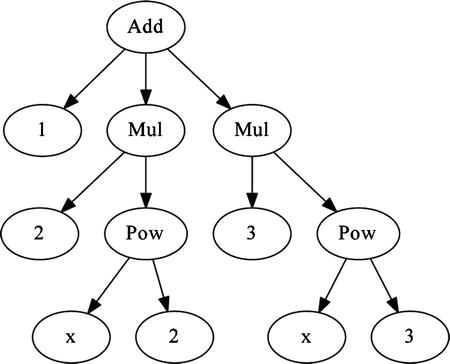
Figure 3-1. Visualization of the expression tree for 1 + 2*x**2 + 3*x**3
The expression tree can be traversed explicitly using the args attribute, which all SymPy operations and symbols provide. For an operator, the args attribute is a tuple of subexpressions that are combined with the rule implemented by the operator class. For symbols, the args attribute is an empty tuple, which signifies that it is a leaf in the expression tree. The following example demonstrates how the expression tree can be explicitly accessed:
In [57]: expr.args
Out[57]: (1, 2x2, 3x3)
In [58]: expr.args[1]
Out[58]: 2x2
In [59]: expr.args[1].args[1]
Out[59]: x2
In [60]: expr.args[1].args[1].args[0]
Out[60]: x
In [61]: expr.args[1].args[1].args[0].args
Out[61]: ()
In basic use of SymPy it is rarely necessary to explicitly manipulate expression trees, but when the methods for manipulating expressions that are introduced in the following section are not sufficient, it is useful to be able to implement functions of your own that traverse and manipulate the expression tree using the args attribute.
Manipulating Expressions
Manipulating expressions trees are one of the main jobs for SymPy, and numerous functions are provided for different types of transformations. The general idea is that expression trees can be transformed between mathematically equivalent forms using simplification and rewrite functions. These functions generally do not change the expression that are passed to the functions, but rather creates a new expression that corresponds to the modified expression. Expressions in SymPy should thus be considered immutable objects (that cannot be changed). All the functions we consider in this section treat SymPy expressions as immutable objects, and return new expression trees rather than modifying expressions in place.
Simplification
The most desirable manipulation of a mathematical expression is to simplify it. This is perhaps and also the most ambiguous operation, since it is nontrivial to determine algorithmically if one expression appears simpler than another to a human being, and in general it is also not obvious which methods should be employed to arrive at a simpler expression. Nonetheless, black-box simplification is an important part of any CAS, and SymPy includes the function sympy.simplify that attempts to simplify a given expression using a variety of methods and approaches. The simplification function can also be invoked through the method simplify, as illustrated in the following example.
In [67]: expr = 2 * (x**2 - x) - x * (x + 1)
In [68]: expr
Out[68]:
In [69]: sympy.simplify(expr)
Out[69]:
In [70]: expr.simplify()
Out[70]:
In [71]: expr
Out[71]:
Note that here both sympy.simplify(expr) and expr.simplify() return new expression trees and leave the expression expr untouched, as mentioned earlier. In this example, the expression expr can be simplified by expanding the products, canceling terms, and then factoring the expression again. In general, sympy.simplify will attempt a variety of different strategies, and will also simplify for example trigonometric and power expressions, as exemplified here:
In [72]: expr = 2 * sympy.cos(x) * sympy.sin(x)
In [73]: expr
Out[73]: 2 sin(x) cos(x)
In [74]: sympy.simplify(expr)
Out[74]: sin(2x)
and
In [75]: expr = sympy.exp(x) * sympy.exp(y)
In [76]: expr
Out[76]: exp(x) exp(y)
In [77]: sympy.simplify(expr)
Out[77]:
Each specific type of simplification can also be carried out with more specialized functions, such as sympy.trigsimp and sympy.powsimp, for trigonometric and power simplifications, respectively. These functions only perform the simplification that their names indicate, and leave other parts of an expression in its original form. A summary of simplification functions in is given in Table 3-3. When the exact simplification steps are known, it is in general better to rely on the more specific simplification functions, since their actions are more well defined and less likely to change in future versions of SymPy. The sympy.simplify function, on the other hand, relies on heuristic approaches that may change in the future, and as a consequence produce different results for a particular input expression.
Table 3-3. Summary of selected SymPy functions for simplifying expressions
|
Function |
Description |
|---|---|
|
sympy.simplify |
Attempt various methods and approaches to obtain a simpler form of a given expression. |
|
sympy.trigsimp |
Attempt to simplify an expression using trigonometric identities. |
|
sympy.powsimp |
Attempt to simplify an expression using laws of powers. |
|
sympy.compsimp |
Simplify combinatorial expressions. |
|
sympy.ratsimp |
Simplify an expression by writing on a common denominator. |
Expand
When the black-box simplification provided by sympy.simplify does not produce satisfying results, it is often possible to make progress by manually guiding SymPy using more specific algebraic operations. An important tool in this process is to expand expression in various ways. The function sympy.expand performs a variety of expansions, depending on the values of optional keyword arguments. By default the function distributes products over additions, into a fully expanded expression. For example, a product of the type ![]() can be expanded to
can be expanded to ![]() using:
using:
In [78]: expr = (x + 1) * (x + 2)
In [79]: sympy.expand(expr)
Out[79]:
Some of the available keyword arguments are mul=True for expanding products (as in the example above), trig=True for trigonometric expansions,
In [80]: sympy.sin(x + y).expand(trig=True)
Out[80]:
log=True for expanding logarithms,
In [81]: a, b = sympy.symbols("a, b", positive=True)
In [82]: sympy.log(a * b).expand(log=True)
Out[82]:
complex=True for separating real and imaginary parts of an expression,
In [83]: sympy.exp(I*a + b).expand(complex=True)
Out[83]:
and power_base=True and power_exp=True for expanding the base and the exponent of a power expression, respectively.
In [84]: sympy.expand((a * b)**x, power_base=True)
Out[84]: axbx
In [85]: sympy.exp((a-b)*x).expand(power_exp=True)
Out[85]:
Calling the sympy.expand function with these keyword arguments set to True is equivalent to calling the more specific functions sympy.expand_mul, sympy.expand_trig, sympy.expand_log, sympy.expand_complex, sympy.expand_power_base, and sympy.expand_power_exp, respectively, but an advantage of the sympy.expand function is that several types of expansions can be performed in a single function call.
Factor, Collect, and Combine
A common use-pattern for the sympy.expand function is to expand an expression, let SymPy cancel terms or factors, and then factor or combine the expression again. The sympy.factor function attempts to factor an expression as far as possible, and is, in some sense, the opposite to sympy.expand with mul=True. It can be used to factor algebraic expressions, such as:
In [86]: sympy.factor(x**2 - 1)
Out[86]:
In [87]: sympy.factor(x * sympy.cos(y) + sympy.sin(z) * x)
Out[87]:
The inverse of the other types of expansions in the previous section can be carried out using sympy.trigsimp, sympy.powsimp, and sympy.logcombine, for example:
In [90]: sympy.logcombine(sympy.log(a) - sympy.log(b))
Out[90]:
When working with mathematical expressions, it is often necessary have fine-grained controlled over factoring. The SymPy function sympy.collect factors terms that contain a given symbol or list of symbols. For example, ![]() cannot be completely factorized, but we can partially factor terms contain x or y:
cannot be completely factorized, but we can partially factor terms contain x or y:
In [89]: expr = x + y + x * y * z
In [90]: expr.collect(x)
Out[90]:
In [91]: expr.collect(y)
Out[91]:
By passing a list of symbols or expressions to the sympy.collect function or to the corresponding collect method, we can collect multiple symbols in one function call. Also, when using the method collect, which returns the new expression, it is possible to chain multiple method calls in the following way:
In [93]: expr = sympy.cos(x + y) + sympy.sin(x - y)
In [94]: expr.expand(trig=True).collect([sympy.cos(x),
    ...:                                 sympy.sin(x)]).collect(sympy.cos(y) - sympy.sin(y))
Out[95]:
Apart, Together, and Cancel
The final type of mathematical simplification that we will consider here is the rewriting of fractions. The functions sympy.apart and sympy.together, which, respectively, rewrite a fraction as a partial fraction, and combine partial fractions to a single fraction, can be used in the following way:
In [95]: sympy.apart(1/(x**2 + 3*x + 2), x)
Out[95]:
In [96]: sympy.together(1 / (y * x + y) + 1 / (1+x))
Out[96]:
In [97]: sympy.cancel(y / (y * x + y))
Out[97]:
In the first example we used sympy.apart to rewrite the expression ![]() as the partial fraction
as the partial fraction
![]() , and we used sympy.together to combine the sum of fractions
, and we used sympy.together to combine the sum of fractions ![]() into an expression on the form of a single fraction. In this example we also used the function sympy.cancel to cancel shared factors between numerator and the denominator in the expression
into an expression on the form of a single fraction. In this example we also used the function sympy.cancel to cancel shared factors between numerator and the denominator in the expression ![]() .
.
Substitutions
The previous sections have been concerned with rewriting expressions using various mathematical identities. Another frequently used form of manipulation of mathematical expressions is substitutions of symbols or subexpressions within an expression. For example, we may want to perform a variable substitution, and replace the variable x with y, or replace a symbol with another expression. In SymPy there are two methods for carrying out substitutions: subs and replace. Usually subs is the most suitable alternative, but in some cases replace provides a more powerful tool, which, for example, can make replacements based on wild card expressions (see docstring for sympy.Symbol.replace for details).
In the most basic use of subs, the method is called on an expression and the symbol or expression that is to be replaced (x) is given as first argument, and the new symbol or the expression (y) is given as second argument. The result is that all occurrences of x in the expression are replaced with y:
In [98]: (x + y).subs(x, y)
Out[98]: 2y
In [99]: sympy.sin(x * sympy.exp(x)).subs(x, y)
Out[99]: sin(yey)
Instead of chaining multiple subs calls when multiple substitutions are required, we can alternatively pass a dictionary as first and only argument to subs, which maps old symbols or expressions to new symbols or expressions:
In [100]: sympy.sin(x * z).subs({z: sympy.exp(y), x: y, sympy.sin: sympy.cos})
Out[100]: cos(yey)
A typical application of the subs method is to substitute numerical values in place of symbolic number, for numerical evaluation (see the following section for more details). A convenient way of doing this is to define a dictionary that translates the symbols to numerical values, and passing this dictionary as argument to the subs method. For example, consider:
In [101]: expr = x * y + z**2 *x
In [102]: values = {x: 1.25, y: 0.4, z: 3.2}
In [103]: expr.subs(values)
Out[103]: 13.3
Numerical Evaluation
Even when working with symbolic mathematics, it is almost invariably sooner or later required to evaluate the symbolic expressions numerically, for example, when producing plots or concrete numerical results. A SymPy expression can be evaluated using either the sympy.N function, or the evalf method of SymPy expression instances:
In [104]: sympy.N(1 + pi)
Out[104]: 4.14159265358979
In [105]: sympy.N(pi, 50)
Out[105]: 3.1415926535897932384626433832795028841971693993751
In [106]: (x + 1/pi).evalf(10)
Out[106]:
Both sympy.N and the evalf method take an optional argument that specifies the number of significant digits to which the expression is to be evaluated, as shown in the previous example where SymPy’s multiprecision float capabilities were leveraged to evaluate the value of π up to 50 digits.
When we need to evaluate an expression numerically for a range of input values, we could in principle loop over the values and perform successive evalf calls, for example:
In [114]: expr = sympy.sin(pi * x * sympy.exp(x))
In [115]: [expr.subs(x, xx).evalf(3) for xx in range(0, 10)]
Out[115]:
However, this method is rather slow, and SymPy provides a more efficient method for doing this operation using the function sympy.lambdify. This function takes a set of free symbols and an expression as arguments, and generates a function that efficiently evaluates the numerical value of the expression. The produced function takes the same number of arguments as the number of free symbols passed as first argument to sympy.lambdify.
In [109]: expr_func = sympy.lambdify(x, expr)
In [110]: expr_func(1.0)
Out[110]: 0.773942685266709
Note that the function expr_func expects numerical (scalar) values as arguments, so we cannot for example pass a symbol, as argument to this function; it is strictly for numerical evaluation. The expr_func created in the previous example is a scalar function, and is not directly compatible with vectorized input in the form of NumPy arrays, as discussed in Chapter 2. However, SymPy is also able to generate functions that are NumPy-array aware: by passing the optional argument 'numpy' as third argument to sympy.lambdify SymPy creates a vectorized function that accepts NumPy arrays as input. This is in general the most efficient way to numerically evaluate symbolic expressions for a large number of input parameters. The following code exemplifies how the SymPy expression expr is converted into a NumPy-array aware vectorized function that can be efficiently evaluated:
In [111]: expr_func = sympy.lambdify(x, expr, 'numpy')
In [112]: import numpy as np
In [113]: xvalues = np.arange(0, 10)
In [114]: expr_func(xvalues)
Out[114]: array([ 0.        ,  0.77394269,  0.64198244,  0.72163867,  0.94361635,
                  0.20523391,  0.97398794,  0.97734066, -0.87034418, -0.69512687])
This is in general an efficient method for generating data from SymPy expressions,2 for example, for plotting and other data oriented applications.
Calculus
So far we have looked at how to represent mathematical expression in SymPy, and how to perform basic simplification and transformation of such expressions. With this framework in place, we are now ready to explore symbolic calculus, or analysis, which is a cornerstone in applied mathematics and has a great number of applications throughout science and engineering. The central concept in calculus is the change of functions as input variables are varied, as quantified by derivatives and differentials; and accumulations of functions over ranges of input, as quantified by integrals. In this section we look at how to compute derivatives and integrals of functions in SymPy.
Derivatives
The derivative of a function describes its rate of change at a given point. In SymPy we can calculate the derivative of a function using sympy.diff, or alternatively by using the diff method of SymPy expression instances. These functions take as argument a symbol, or a number of symbols, for which the function or the expression is to be derived with respect to. To represent the first order derivative of an abstract function f(x) with respect to x, we can do
In [119]: f = sympy.Function('f')(x)
In [120]: sympy.diff(f, x)               # equivalent to f.diff(x)
Out[120]:
and to represent higher-order derivatives, all we need to do is to repeat the symbol x in the argument list in the call to sympy.diff, or equivalently by specifying an integer as an argument following a symbol, which defines the number of times the expression should be derived with respect to that symbol:
In [117]: sympy.diff(f, x, x)
Out[117]:
In [118]: sympy.diff(f, x, 3)       # equivalent to sympy.diff(f, x, x, x)
Out[118]:
This method is readily extended to multivariate functions:
In [119]: g = sympy.Function('g')(x, y)
In [120]: g.diff(x, y)               # equivalent to sympy.diff(g, x, y)
Out[120]:
In [121]: g.diff(x, 3, y, 2)         # equivalent to sympy.diff(g, x, x, x, y, y)
Out[121]:
These examples so far only involve formal derivatives of undefined functions. Naturally, we can also evaluate the derivatives of defined functions and expressions, which result in new expressions that correspond to the evaluated derivatives. For example, using sympy.diff we can easily evaluate derivatives of arbitrary mathematical expressions, such as polynomials:
In [122]: expr = x**4 + x**3 + x**2 + x + 1
In [123]: expr.diff(x)
Out[123]:
In [124]: expr.diff(x, x)
Out[124]: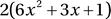
In [125]: expr = (x + 1)**3 * y ** 2 * (z - 1)
In [126]: expr.diff(x, y, z)
Out[126]:
as well as trigonometric and other more complicated mathematical expressions:
In [127]: expr = sympy.sin(x * y) * sympy.cos(x / 2)
In [128]: expr.diff(x)
Out[128]:
In [129]: expr = sympy.special.polynomials.hermite(x, 0)
In [130]: expr.diff(x).doit()
Out[130]: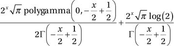
Derivatives are usually relatively easy to compute, and sympy.diff should be able to evaluate the derivative of most standard mathematical functions defined in SymPy.
Note that in these examples, calling sympy.diff on an expression directly results in a new expression. If we want instead to symbolically represent the derivative of a definite expression, we can create an instance of the class sympy.Derivative, passing the expression as first argument, followed by the symbols with respect to the derivative that is to be computed:
In [131]: d = sympy.Derivative(sympy.exp(sympy.cos(x)), x)
In [132]: d
Out[132]:
This formal representation of a derivative can then be evaluated by calling the doit method on the sympy.Derivative instance:
In [133]: d.doit()
Out[133]:
This pattern of delayed evaluation is reoccurring throughout SymPy, and full control of when a formal expression is evaluated to a specific result is useful in many situations, in particular with expressions that can be simplified or manipulated while represented as a formal expression rather than after it has been evaluated.
Integrals
In SymPy, integrals are evaluated using the function sympy.integrate, and formal integrals can be represented using sympy.Integral (which, as the case with sympy.Derviative, can be explicitly evaluated by calling the doit method). Integrals come in two basic forms: definite and indefinite, where a definite integral has specified integration limits, and can be interpreted as an area or volume; while an indefinite integral does not have integration limits, and denotes the antiderivative (inverse of the derivative of a function). SymPy handles both indefinite and definite integrals using the sympy.integrate function.
If the sympy.integrate function is called with only an expression as argument, the indefinite integral is computed. On the other hand, a definite integral is computed if the sympy.integrate function additionally is passed a tuple on the form (x, a, b), where x is the integration variable and a and b are the integration limits. For a single-variable function f (x), the indefinite and definite integrals are therefore computed using:
In [135]: a, b, x, y = sympy.symbols("a, b, x, y")
     ...: f = sympy.Function("f")(x)
In [136]: sympy.integrate(f)
Out[136]:
In [137]: sympy.integrate(f, (x, a, b))
Out[137]:
and when these methods are applied to explicit functions the integrals are evaluated accordingly:
In [138]: sympy.integrate(sympy.sin(x))
Out[138]:
In [139]: sympy.integrate(sympy.sin(x), (x, a, b))
Out[139]:
Definite integrals can also include limits that extend from negative infinity, and/or to positive infinite, using SymPy’s symbol for infinity oo:
In [139]: sympy.integrate(sympy.exp(-x**2), (x, 0, oo))
Out[139]:
In [140]: a, b, c = sympy.symbols("a, b, c", positive=True)
In [141]: sympy.integrate(a * sympy.exp(-((x-b)/c)**2), (x, -oo, oo))
Out[141]:
Computing integrals symbolically is in general a difficult problem, and SymPy will not be able to give symbolic results for any integral you can come up with. When SymPy fails to evaluate an integral, an instance of sympy.Integral, representing the formal integral, is returned instead.
In [142]: sympy.integrate(sympy.sin(x * sympy.cos(x)))
Out[142]:
Multivariable expression can also be integrated with sympy.integrate. In the case of indefinite integral of a multivariable expression, the integration variable has to be specified explicitly:
In [140]: expr = sympy.sin(x*sympy.exp(y))
In [141]: sympy.integrate(expr, x)
Out[141]:
In [142]: expr = (x + y)**2
In [143]: sympy.integrate(expr, x)
Out[143]:
By passing more than one symbol, or more than one tuple that contain symbols and their integration limits, we can carry out multiple integration:
In [144]: sympy.integrate(expr, x, y)
Out[144]:
In [145]: sympy.integrate(expr, (x, 0, 1), (y, 0, 1))
Out[145]:
Series
Series expansions are an important tool in many disciplines in computing. With a series expansion, an arbitrary function can be written as a polynomial, with coefficients given by the derivatives of the function at the point around which the series expansion is made. By truncating the series expansion at some order n, the nth order approximation of the function is obtained. In SymPy, the series expansion of a function or an expression can be computed using the function sympy.series or the series method available in SymPy expression instances. The first argument to sympy.series is a function or expression that is to be expanded, followed by a symbol with respect to which the expansion is to be computed (it can be omitted for single-variable expressions and function). In addition, it is also possible to request a particular point around which the series expansions is to be performed (using the x0 keyword argument, with default x0 = 0), specifying the order of the expansion (using the n keyword argument, with default n = 6), and specifying the direction from which the series is computed, that is, from below or above x0 (using the dir keyword argument, which defaults to dir ='+').
For an undefined function f (x), the expansion up to sixth order around x0 = 0 is computed using:
In [147]: x = sympy.Symbol("x")
In [148]: f = sympy.Function("f")(x)
In [149]: sympy.series(f, x)
Out[149]:
To change the point around which the function is expanded, we specify the x0 argument as in the following example:
In [147]: x0 = sympy.Symbol("{x_0}")
In [151]: f.series(x, x0, n = 2)
Out[151]:
Here we also specified n = 2, to request a series expansion with only terms up to second order. Note that the errors due to the truncated terms are represented by the order object ![]() . The order object is useful for keeping track of the order of an expression when computing with series expansions, such as multiplying or adding different expansions. However, for concrete numerical evolution, it is necessary to remove the order term from the expression, which can be done using the method removeO:
. The order object is useful for keeping track of the order of an expression when computing with series expansions, such as multiplying or adding different expansions. However, for concrete numerical evolution, it is necessary to remove the order term from the expression, which can be done using the method removeO:
In [152]: f.series(x, x0, n = 2).removeO()
Out[152]:
While the expansions shown above were computed for an unspecified function f (x), we can naturally also compute the series expansions of specific functions and expressions, and in those cases we obtain specific evaluated results. For example, we can easily generate the well-known expansions of many standard mathematical functions:
In [153]: sympy.cos(x).series()
Out[153]:
In [154]: sympy.sin(x).series()
Out[154]:
In [155]: sympy.exp(x).series()
Out[155]:
In [156]: 1/(1+x)).series()
Out[156]:
as well as arbitrary expressions of symbols and functions, which in general can also be multivariable functions:
In [157]: expr = sympy.cos(x) / (1 + sympy.sin(x * y))
In [158]: expr.series(x, n = 4)
Out[158]:
In [159]: expr.series(y, n = 4)
Out[159]:
Limits
Another important tool in calculus is limits, which denotes the value of a function as one of its dependent variables approaches a specific value, or as the value of the variable approach negative or positive infinity. An example of a limit is one of the definitions of the derivative:
![]()
While limits are more of a theoretical tool, and do not have as many practical applications as, say, series expansions, it is still useful to be able to compute limits using SymPy. In SymPy, limits can be evaluated using the sympy.limit function, which takes an expression, a symbol it depends on, as well as the value that the symbol approaches in the limit. For example, to compute the limit of the function sin(x)/x, as the variable x goes to zero, that is ![]() , we can use:
, we can use:
In [161]: sympy.limit(sympy.sin(x) / x, x, 0)
Out[161]: 1
Here we obtained the well-known answer 1 for this limit. We can also use sympy.limit to compute symbolic limits, which can be illustrated by computing derivatives using the previous definition (although it is, of course, more efficient to use sympy.diff),
In [162]: f = sympy.Function('f')
     ...: x, h = sympy.symbols("x, h")
In [163]: diff_limit = (f(x + h) - f(x))/h
In [164]: sympy.limit(diff_limit.subs(f, sympy.cos), h, 0)
Out[164]:
In [165]: sympy.limit(diff_limit.subs(f, sympy.sin), h, 0)
Out[165]: cos(x)
A more practical example of using limits is to find the asymptotic behavior as a function, for example as its dependent variable approach infinity. As an example, consider the function ![]() and suppose we are interested in the large-x dependence of this function. It will be on the form
and suppose we are interested in the large-x dependence of this function. It will be on the form ![]() , and we can compute p and q using sympy.limit as in the following:
, and we can compute p and q using sympy.limit as in the following:
In [166]: expr = (x**2 - 3*x) / (2*x - 2)
In [167]: p = sympy.limit(expr/x, x, sympy.oo)
In [168]: q = sympy.limit(expr - p*x, x, sympy.oo)
In [169]: p, q
Out[169]:
Thus, the asymptotic behavior of f (x) as x becomes large is the linear function ![]() .
.
Sums and Products
Sums and products can be symbolically represented using the SymPy classes sympy.Sum and sympy.Product. They both take an expression as their first argument, and as a second argument they take a tuple of the form (n, n1, n2), where n is a symbol and n1 and n2 are the lower and upper limits for the symbol n, in the sum or product, respectively. After sympy.Sum or sympy.Product objects have been created, they can be evaluated using the doit method:
In [171]: n = sympy.symbols("n", integer=True)
In [172]: x = sympy.Sum(1/(n**2), (n, 1, oo))
In [173]: x
Out[173]:
In [174]: x.doit()
Out[174]:
In [175]: x = sympy.Product(n, (n, 1, 7))
In [176]: x
Out[176]:
In [177]: x.doit()
Out[177]: 5040
Note that the sum in the previous example was specified with an upper limit of infinity. It is therefore clear that this sum was not evaluated by explicit summation, but was rather computed analytically. SymPy can evaluate many summations of this type, including when the summand contains symbolic variables other than the summation index, such as in the following example:
In [178]: x = sympy.Symbol("x")
In [179]: sympy.Sum((x)**n/(sympy.factorial(n)), (n, 1, oo)).doit().simplify()
Out[179]:
Equations
Equation solving is a fundamental part of mathematics with applications in nearly every branch of science and technology, and it is therefore immensely important. SymPy can solve a wide variety of equations symbolically, although many equations cannot be solved analytically even in principle. If an equation, or a system or equations, can be solved analytically, there is a good chance that SymPy is able to find the solution. If not, numerical methods might be the only option.
In its simplest form, equation solving involves a single equation with a single unknown variable, and no additional parameters: for example, finding the value of x that satisfy the second-degree polynomial equation ![]() . This equation is of course easy to solve, even by hand, but in SymPy we can use the function sympy.solve to find the solutions of x that satisfy this equation using:
. This equation is of course easy to solve, even by hand, but in SymPy we can use the function sympy.solve to find the solutions of x that satisfy this equation using:
In [170]: x = sympy.Symbol("x")
In [171]: sympy.solve(x**2 + 2*x - 3)
Out[171]:
That is, the solutions are x = –3 and x = 1. The argument to the sympy.solve function is an expression that will be solved under the assumption that it equals zero. When this expression contains more than one symbol, the variable that is to be solved for must be given as a second argument. For example,
In [172]: a, b, c = sympy.symbols("a, b, c")
In [173]: sympy.solve(a * x**2 + b * x + c, x)
Out[173]:
and in this case the resulting solutions are expressions that depend on the symbols representing the parameters in the equation.
The sympy.solve function is also capable of solving other types of equations, for example including trigonometric expressions:
In [174]: sympy.solve(sympy.sin(x) - sympy.cos(x), x)
Out[174]:
and equations whose solution can be expressed in terms of special functions:
In [180]: sympy.solve(sympy.exp(x) + 2 * x, x)
Out[180]:
However, when dealing with general equations, even in for a univariate case, it is not uncommon to encounter equations that are not solvable algebraically, or that SymPy is unable to solve. In these cases SymPy will return a formal solution, which can be evaluated numerically if needed, or raise an error if no method is available for that particular type of equation:
In [176]: sympy.solve(x**5 - x**2 + 1, x)
Out[176]:

In [177]: sympy.solve(sympy.tan(x) + x, x)
---------------------------------------------------------------------------
NotImplementedError                       Traceback (most recent call last)
...
NotImplementedError: multiple generators [x, tan(x)] No algorithms are implemented to solve equation x + tan(x)
Solving a system of equations for more than one unknown variable in SymPy is a straightforward generalization of the procedure used for univariate equations. Instead of passing a single expression as first argument to sympy.solve, a list of expressions that represent the system of equations is used, and in this case the second argument should be a list of symbols to solve for. For example, the following two examples demonstrate how to solve two systems that are linear and nonlinear equations in x and y, respectively:
In [178]: eq1 = x + 2 * y – 1
...: eq2 = x - y + 1
In [179]: sympy.solve([eq1, eq2], [x, y], dict=True)
Out[179]: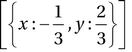
In [180]: eq1 = x**2 - y
...: eq2 = y**2 - x
In [181]: sols = sympy.solve([eq1, eq2], [x, y], dict=True)
In [182]: sols
Out[182]:
Note that in both these examples, the function sympy.solve returns a list where each element represents a solution to the equation system. The optional keyword argument dict = True was also used, to request that each solution is return in dictionary format, which maps the symbols that have been solved for to their values. This dictionary can conveniently be used in, for example, calls to subs, which is used in the following code that checks that each solution indeed satisfies the two equations:
In [183]: [eq1.subs(sol).simplify() == 0 and eq2.subs(sol).simplify() == 0 for sol in sols]
Out[183]: [True, True, True, True]
Linear Algebra
Linear algebra is another fundamental branch of mathematics with important applications throughout scientific and technical computing. It concerns vectors, vector spaces, and linear mappings between vector spaces, which can be represented as matrices. In SymPy we can represent vectors and matrices symbolically using the sympy.Matrix class, whose elements can in turn be represented by numbers, symbols, or even arbitrary symbolic expressions. To create a matrix with numerical entries we can, as in the case of NumPy arrays in Chapter 2, pass a Python list to sympy.Matrix:
In [184]: sympy.Matrix([1,2])
Out[184]:
In [185]: sympy.Matrix([[1,2]])
Out[185]:
In [186]: sympy.Matrix([[1, 2], [3, 4]])
Out[186]:
As this example demonstrates, a single list generates a column vector, while a matrix requires a nested list of values. Note that unlike the multidimensional arrays in NumPy discussed in Chapter 2, the sympy.Matrix object in SymPy is only for two-dimensional arrays, that is, matrices. Another way of creating new sympy.Matrix objects is to pass as arguments the number of rows, the number of columns, and a function that takes the row and column index as arguments and returns the value of the corresponding element:
In [187]: sympy.Matrix(3, 4, lambda m, n: 10 * m + n)
Out[187]:
The most powerful features of SymPy’s matrix objects, which distinguish it from for example NumPy arrays, are of course that its elements themselves can be symbolic expressions. For example, an arbitrary 2x2 matrix can be represented with a symbolic variable for each of its elements:
In [188]: a, b, c, d = sympy.symbols("a, b, c, d")
In [189]: M = sympy.Matrix([[a, b], [c, d]])
In [190]: M
Out[190]:
and such matrices can naturally also be used in computations, which then remains parameterized with the symbolic values of the elements. The usual arithmetic operators are implemented for matrix objects, but note that multiplication operator * in this case denotes matrix multiplication:
In [191]: M * M
Out[191]:
In [192]: x = sympy.Matrix(sympy.symbols("x_1, x_2"))
In [194]: M * x
Out[194]:
In addition to arithmetic operations, many standard linear algebra operations on vectors and matrices are also implemented as SymPy functions and methods of the sympy.Matrix class. Table 3-4 gives a summary of frequently used linear-algebra related functions (see the docstring for sympy.Matrix for a complete list), and SymPy matrices can also be operated in an element-oriented fashion using indexing and slicing operations that closely resembles those discussed for NumPy arrays in Chapter 2.
Table 3-4. Selected functions and methods for operating on SymPy matrices
|
Function / Method |
Description |
|---|---|
|
transpose / T |
Compute the transpose of a matrix. |
|
adjoint / H |
Compute the adjoint of a matrix. |
|
trace |
Compute the trace (sum of diagonal elements) of a matrix. |
|
det |
Compute the determinant of a matrix. |
|
inv |
Compute the inverse of a matrix. |
|
LUdecomposition |
Compute the LU decomposition of a matrix. |
|
LUsolve |
Solve a linear system of equations on the form |
|
QRdecomposition |
Compute the QR decomposition of a matrix. |
|
QRsolve |
Solve a linear system of equations on the form |
|
diagonalize |
Diagonalize a matrix M, such that it can be written on the form |
|
norm |
Compute the norm of a matrix. |
|
nullspace |
Compute a set of vectors that spans the null space of a matrix. |
|
rank |
Compute the rank of a matrix. |
|
singular_values |
Compute the singular values of a matrix. |
|
solve |
Solve a linear system of equations on the form |
As an example of a problem that can be solved with symbolic linear algebra using SymPy, but which is not directly solvable with purely numerical approaches, consider the following parameterized linear equation system:
![]()
![]()
which we would like to solve for the unknown variables x and y. Here p, q, b1 and b2 are unspecified parameters. On matrix form, we can write these two equations as

With purely numerical methods, we would have to choose particular values of the parameters p and q before we could begin to solve this problem, for example, using an LU factorization (or by computing the inverse) of the matrix on the left-hand side of the equation. With a symbolic computing approach, on the other hand, we can directly proceed with computing the solution, as if we carried out the calculation analytically by hand. With SymPy, we can simply define symbols for the unknown variables and parameters, and setup the required matrix objects:
In [195]: p, q = sympy.symbols("p, q")
In [196]: M = sympy.Matrix([[1, p], [q, 1]])
In [203]: M
Out[203]:
In [197]: b = sympy.Matrix(sympy.symbols("b_1, b_2"))
In [198]: b
Out[198]:
and then use, for example, the LUsolve method to solve the linear equation system:
In [199]: x = M.LUsolve(b)
In [200]: x
Out[200]:
Alternatively, we could also directly compute the inverse of the matrix M, and multiply it with the vector b:
In [201]: x = M.inv() * b
In [202]: x
Out[202]: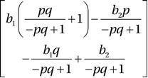
However, computing the inverse of a matrix is more difficult than performing the LU factorization, so if solving the equation ![]() is the objective, as it was here, then using LU factorization is more efficient. This becomes particularly noticeable for larger equation systems. With both methods considered here, we obtain a symbolic expression for the solution that is trivial to evaluate for any parameter values, without having to recompute the solution. This is the strength of symbolic computing, and an example of how it sometimes can excel over direct numerical computing. The example considered here could of course also be solved easily by hand, but as the number of equations and unspecified parameters grow, analytical treatment by hand quickly becomes prohibitively lengthy and tedious. With the help of a computer algebra system such as SymPy, we can push the limits of which problems can be treated analytically.
is the objective, as it was here, then using LU factorization is more efficient. This becomes particularly noticeable for larger equation systems. With both methods considered here, we obtain a symbolic expression for the solution that is trivial to evaluate for any parameter values, without having to recompute the solution. This is the strength of symbolic computing, and an example of how it sometimes can excel over direct numerical computing. The example considered here could of course also be solved easily by hand, but as the number of equations and unspecified parameters grow, analytical treatment by hand quickly becomes prohibitively lengthy and tedious. With the help of a computer algebra system such as SymPy, we can push the limits of which problems can be treated analytically.
Summary
This chapter introduced computer-assisted symbolic computing using Python and the SymPy library. Although analytical and numerical techniques are often considered separately, it is a fact that analytical methods underpin everything in computing, and are essential in developing algorithms and numerical methods. Whether analytical mathematics is carried by hand, or using a computer algebra system such as SymPy, it is an essential tool for computational work. The view and approach that I would like to encourage is therefore the following: analytical and numerical methods are closely intertwined, and it is often worthwhile to start analyzing a computational problem with analytical and symbolic methods. When such methods turn out to be unfeasible, it is time to resort to numerical methods. However, by directly applying numerical methods to a problem, before analyzing it analytically, it is likely that one ends up solving a more difficult computational problem than is really necessary.
Further Reading
For a quick and short introduction to SymPy, see, for example, Instant SymPyStarter. The official SymPy documentation also provides a great tutorial for getting started with SymPy. It is available at http://docs.sympy.org/latest/tutorial/index.html.
References
Lamy, R. (2013). Instant SymPy Starter. Mumbai: Packt.
____________________
1Here it is important to keep in mind the distinction between a Python function, or callable Python object such as sympy.Function, and the symbolic function that a sympy.Function class instance represents.
2See also the ufuncity from the sympy.utilities.autowrap module and the theano_function from the sympy.printing.theanocode module. These provide similar functionality as sympy.lambdify, but using different computational back ends.