![]()
Data Processing and Analysis
In the last several chapters we have covered the main topics of traditional scientific computing. These topics provide a foundation for most computational work. Starting with this chapter, we move on to explore data processing and analysis, statistics, and statistical modeling. As a first step in this direction, we look at the data analysis library pandas. This library provides convenient data structures for representing series and tables of data, and makes it easy to transform, split, merge, and convert data. These are important steps in the process1 of cleansing raw data into a tidy form that is suitable for analysis. The pandas library builds on top of NumPy, and complements it with features that are particularly useful when handling data, such as labeled indexing, hierarchical indices, alignment of data for comparison and merging of datasets, handling of missing data, and much more. As such, the pandas library has become a de facto library for high-level data processing in Python, especially for statistics applications. The pandas library itself contains only limited support for statistical modeling (namely, linear regression). For more involved statistical analysis and modeling there are other packages available, such as statmodels, patsy, and scikit-learn, which we cover in later chapters. However, also for statistical modeling with these packages, pandas can still be used for data representation and preparation. The pandas library is therefore a key component in the software stack for data analysis with Python.
![]() pandas The pandas library is a framework for data processing and analysis in Python. At the time of writing, the most recent version of pandas is 0.16.2. For more information about the pandas library, and its official documentation, see the project’s web site at http://pandas.pydata.org.
pandas The pandas library is a framework for data processing and analysis in Python. At the time of writing, the most recent version of pandas is 0.16.2. For more information about the pandas library, and its official documentation, see the project’s web site at http://pandas.pydata.org.
The main focus of this chapter is to introduce basic features and usage of the pandas library. Toward the end of the chapter we also briefly explore the statistical visualization library seaborn, which is built on top of Matplotlib. This library provides quick and convenient graphing of data represented as pandas data structure (or NumPy arrays). Visualization is a very important part of exploratory data analysis, and the pandas library itself also provides functions for basic data visualization (which also builds on top of Matplotlib). The seaborn library takes this further, by providing additional statistical graphing capabilities and improved styling: The seaborn library is notable for generating good-looking graphics using defaults settings.
![]() seaborn The seaborn library is a visualization library for statistical graphics. It builds on Matplotlib and provides easy-to-use functions for common statistical graphs. At the time of writing, the most recent version of seaborn is 0.6.0. For more information about seaborn, and its official documentation, see the project’s web site at: http://stanford.edu/~mwaskom/software/seaborn.
seaborn The seaborn library is a visualization library for statistical graphics. It builds on Matplotlib and provides easy-to-use functions for common statistical graphs. At the time of writing, the most recent version of seaborn is 0.6.0. For more information about seaborn, and its official documentation, see the project’s web site at: http://stanford.edu/~mwaskom/software/seaborn.
Importing Modules
In this chapter we mainly work with the pandas library, which we assume is imported under the name pd:
In [1]: import pandas as pd
We also require NumPy and Matplotlib, which we import as usual in the following way:
In [2]: import numpy as np
In [3]: import matplotlib.pyplot as plt
For more aesthetically pleasing default appearances of Matplotlib figures produced by the pandas library, we select an improved default style using the pandas function set_option:
In [4]: pd.set_option('display.mpl_style', 'default')
Later in this chapter we will also require to import the seaborn module, which we will import under the name sns, but for now we do not import this library since it alters the default appearance of graphics generated with Matplotlib.
Introduction to Pandas
The main focus of this chapter is the pandas library for data analysis, and we begin here with an introduction to this library. The pandas library mainly provides data structures and methods for representing and manipulating data. The two main data structures in pandas are the Series and DataFrame objects, which are used to represent data series and tabular data, respectively. Both of these objects have an index for accessing elements or rows in the data represented by the object. By default, the indices are integers starting from zero, like NumPy arrays, but it is also possible to use as index any sequence of identifiers.
Series
The merit of being able to index a data series with labels rather than integers is apparent even in the simplest of examples: Consider the following construction of a Series object. We give the constructor a list of integers, to create a Series object that represents the given data. Displaying the object in IPython reveals the data of the Series object together with the corresponding indices:
In [5]: s = pd.Series([909976, 8615246, 2872086, 2273305])
In [6]: s
Out[6]: 0     909976
        1     8615246
        2     2872086
        3     2273305
        dtype: int64
The resulting object is a Series instance with data type (dtype) int64, and the elements are indexed by the integers 0, 1, 2, and 3. Using the index and values attributes, we can extract the underlying data for the index and the values stored in the series:
In [7]: s.index
Out[7]: Int64Index([0, 1, 2, 3], dtype='int64')
In [8]: s.values
Out[8]: array([ 909976, 8615246, 2872086, 2273305])
While using integer-indexed arrays or data series is a fully functional representation of the data, it is not descriptive. For example, if the data represents the population of four European capitals, it is convenient and descriptive to use the city names as indices rather than integers. With a Series object this is possible, and we can assign the index attribute of a Series object to a list with new indices to accomplish this. We can also set the name attribute of the Series object, to give it a descriptive name:
In [9]: s.index = ["Stockholm", "London", "Rome", "Paris"]
In [10]: s.name = "Population"
In [11]: s
Out[11]: Stockholm     909976
         London       8615246
         Rome         2872086
         Paris        2273305
         Name: Population, dtype: int64
It is now immediately obvious what the data represents. Alternatively, we can also set the index and name attributes through keyword arguments to the Series object when it is created:
In [12]: s = pd.Series([909976, 8615246, 2872086, 2273305], name="Population",
    ...:               index=["Stockholm", "London", "Rome", "Paris"])
While it is perfectly possible to store the data for the populations of these cities directly in a NumPy array, even in this simple example it is much clearer what the data represent when the data points are indexed with meaningful labels. The benefits of bringing the description of the data closer to the data are even greater when the complexity of the dataset increases.
We can access elements in a Series by indexing with the corresponding index (label), or directly through an attribute with the same name as the index (if the index label is a valid Python symbol name):
In [13]: s["London"]
Out[13]: 8615246
In [14]: s.Stockholm
Out[14]: 909976
Indexing a Series object with a list of indices gives a new Series object with a subset of the original data (corresponding to the provided list of indices):
In [15]: s[["Paris", "Rome"]]
Out[15]: Paris    2273305
         Rome     2872086
         Name: Population, dtype: int64
With a data series represented as a Series object, we can easily compute its descriptive statistics using the Series methods count (the number of data points), median (calculate the median), mean (calculate the mean value), std (calculate the standard deviation), min and max (minimum and maximum value), and the quantile (for calculating quantiles):
In [16]: s.median(), s.mean(), s.std()
Out[16]: (2572695.5, 3667653.25, 3399048.5005155364)
In [17]: s.min(), s.max()
Out[17]: (909976, 8615246)
In [18]: s.quantile(q=0.25), s.quantile(q=0.5), s.quantile(q=0.75)
Out[18]: (1932472.75, 2572695.5, 4307876.0)
All of the above are combined in the output of the describe method, which provides a summary of the data represented by a Series object:
In [19]: s.describe()
Out[19]: count          4.000000
         mean     3667653.250000
         std      3399048.500516
         min       909976.000000
         25%      1932472.750000
         50%      2572695.500000
         75%      4307876.000000
         max      8615246.000000
         Name: Population, dtype: float64
Using the plot method, we can quickly and easily produce graphs that visualize the data in a Series object. The pandas library uses Matplotlib to produce graphs, and we can optionally pass a Matplotlib Axes instance to the plot method via the ax argument. The type of the graph is specified using the kind argument (valid options are line, hist, bar, barh, box, kde, density, area and pie). See Figure 12-1.
In [20]: fig, axes = plt.subplots(1, 4, figsize=(12, 3))
    ...: s.plot(ax=axes[0], kind='line', title='line')
    ...: s.plot(ax=axes[1], kind='bar', title='bar')
    ...: s.plot(ax=axes[2], kind='box', title='box')
    ...: s.plot(ax=axes[3], kind='pie', title='pie')

Figure 12-1. Examples of plot styles that can be produced with pandas using the Series.plot method
DataFrame
As we have seen in the previous examples, a pandas Series object provides a convenient container for one-dimensional arrays, which can use descriptive labels for the elements, and which provides quick access to descriptive statistics and visualization. For higher-dimensional arrays (mainly two-dimensional arrays or tables), the corresponding data structure is the pandas DataFrame object. It can be viewed as a collection of Series objects with a common index.
There are numerous ways to initialize a DataFrame. For simple examples, the easiest way is to pass a nested Python list or dictionary to the constructor of the DataFrame object. For example, consider an extension of the dataset we used in the previous section, where in addition to the population of each city we also include a column that specifies which state each city belongs to. We can create the corresponding DataFrame object in the following way:
In [21]: df = pd.DataFrame([[909976, "Sweden"],
    ...:                    [8615246, "United Kingdom"],
    ...:                    [2872086, "Italy"],
    ...:                    [2273305, "France"]])
In [22]: df
Out[22]:
              0         1
         0    909976    Sweden
         1    8615246   United Kingdom
         2    2872086   Italy
         3    2273305   France
The result is tabular data structure with rows and columns. Like with a Series object, we can use labeled indexing for rows by assigning a sequence of labels to the index attribute, and, in addition, we can set the columns attribute to a sequence of labels for the columns:
In [23]: df.index = ["Stockholm", "London", "Rome", "Paris"]
In [24]: df.columns = ["Population", "State"]
In [25]: df
Out[25]:
                      Population    State

         Stockholm    909976        Sweden

         London       8615246       United Kingdom

         Rome         2872086       Italy

         Paris        2273305       France
The index and columns attributes can also be set using the corresponding keyword arguments to the DataFrame object when the it is created:
In [26]: df = pd.DataFrame([[909976, "Sweden"],
    ...:                    [8615246, "United Kingdom"],
    ...:                    [2872086, "Italy"],
    ...:                    [2273305, "France"]],
    ...:                   index=["Stockholm", "London", "Rome", "Paris"],
    ...:                   columns=["Population", "State"])
An alternative way to create the same data frame, which sometimes can be more convenient, is to pass a dictionary with column titles as keys and column data as values:
In [27]: df = pd.DataFrame({"Population": [909976, 8615246, 2872086, 2273305],
    ...:                    "State": ["Sweden", "United Kingdom", "Italy", "France"]},
    ...:                   index=["Stockholm", "London", "Rome", "Paris"])
As before, the underlying data in a DataFrame can be obtained as a NumPy array using the values attribute, and the index and column arrays through the index and columns attributes, respectively. Each column in a data frame can be accessed using the column name as attribute (or, alternatively, by indexing with the column label, for example df["Population"]):
In [28]: df.Population
Out[28]: Stockholm     909976
         London       8615246
         Rome         2872086
         Paris        2273305
         Name: Population, dtype: int64
The result of extracting a column from a DataFrame is a new Series object, which we can process and manipulate with the methods discussed in the previous section. Rows of a DataFrame instance can be accessed using the ix indexer attribute. Indexing this attribute also results in a Series object, which corresponds to a row of the original data frame:
In [29]: df.ix["Stockholm"]
Out[29]: Population    909976
         State         Sweden
         Name: Stockholm, dtype: object
Passing a list of row labels to the ix indexer results in a new DataFrame that is a subset of the original DataFrame, containing only the selected rows:
In [30]: df.ix[["Paris", "Rome"]]
Out[30]:
                   Population   State

         Paris     2273305      France

         Rome      2872086      Italy
The ix indexer can also be used to select both rows and columns simultaneously, by passing first a row label (or list thereof), and second a column label (or list thereof). The result is a DataFrame, a Series, or an element value, depending on the number of columns and rows that are selected:
In [31]: df.ix[["Paris", "Rome"], "Population"]
Out[31]: Paris    2273305
         Rome     2872086
         Name: Population, dtype: int64
We can compute descriptive statistics using the same methods as we already used for Series objects. When invoking those methods (mean, std, median, min, max, etc.) for a DataFrame, the calculation is performed for each column with numerical data types:
In [32]: df.mean()
Out[32]: Population    3667653.25
         dtype: float64
In this case, only one of the two columns has a numerical data type (the one named Population). Using the DataFrame method info and the attribute dtype, we can obtain a summary of the content in a DataFrame, and the data types of each column:
In [33]: df.info()
<class 'pandas.core.frame.DataFrame'>
Index: 4 entries, Stockholm to Paris
Data columns (total 2 columns):
Population    4 non-null int64
State         4 non-null object
dtypes: int64(1), object(1)
memory usage: 96.0+ bytes
In [34]: df.dtypes
Out[34]: Population     int64
         State         object
         dtype: object
The real advantages of using pandas emerge when dealing with larger and more complex datasets than the examples we have used so far. Such data can rarely be defined as explicit lists or dictionaries, which can be passed to the DataFrame initializer. A more common situation is that the data must be read from a file, or some other external source. The pandas library supports numerous methods for reading data from files of different formats. Here we use the read_csv function to read in data and create a DataFrame object from a CSV file.2 This function accepts a large number of optional arguments for tuning its behavior. See the docstring help(pd.read_csv) for details. Some of the most useful arguments are header (specifies which row, if any, contains a header with column names), skiprows (number of rows to skip before starting to read data, or a list of line numbers of lines to skip), delimiter (the character that is used as a delimiter between column values), encoding (the name of the encoding used in the file, for example utf-8), and nrows (number of rows to read). The first and only mandatory argument to the pd.read_csv function is a filename or an URL to the data source. For example, to read in a dataset stored in a file called european_cities.csv3, of which the first five lines are show below, we can simply call pd.read_csv("european_cities.csv"), since the default delimiter is "," and the header is by default taken from the first line. However, we could also write out all these options explicitly:
In [35]: !head –n 5 european_cities.csv
Rank,City,State,Population,Date of census
1,London, United Kingdom,"8,615,246",1 June 2014
2,Berlin, Germany,"3,437,916",31 May 2014
3,Madrid, Spain,"3,165,235",1 January 2014
4,Rome, Italy,"2,872,086",30 September 2014
In [36]: df_pop = pd.read_csv("european_cities.csv",
    ...:                      delimiter=",", encoding="utf-8", header=0)
This dataset is similar to the example data we used earlier in this chapter, but here there are additional columns and many more rows for other cities. Once a dataset is read into a DataFrame object, it is useful to start by inspecting the summary given by the info method, to begin forming an idea of the properties of the dataset.
In [37]: df_pop.info()
<class 'pandas.core.frame.DataFrame'>
Int64Index: 105 entries, 0 to 104
Data columns (total 5 columns):
Rank              105 non-null int64
City              105 non-null object
State             105 non-null object
Population        105 non-null object
Date of census    105 non-null object
dtypes: int64(1), object(4) memory usage: 4.9+ KB
Here we see that there are 105 rows in this dataset, and that it has five columns. Only the Rank column is of numerical data type. In particular, the Population column is not yet of numeric data type because its values are of the format "8,615,246," and is therefore interpreted as string values by the read_csv function. It is also informative to display a tabular view of the data. However, this dataset is too large to display in full, and in situations like this the head and tail methods are handy for creating a truncated dataset containing the first few and last few rows, respectively. Both of these functions take an optional argument that specifies how many rows to include in the truncated DataFrame. Note also that df.head(n) is equivalent to df[:n], where n is an integer.

Displaying a truncated DataFrame gives a good idea of how the data looks, and what remains to be done before the data is ready for analysis. It is common to have to transform columns in one way or another, and to reorder the table by sorting by a specific column, or by ordering the index. In the following we explore some methods for modifying DataFrame objects. First of all, we can create new columns and update columns in a DataFrame simply by assigning a Series object to the DataFrame indexed by the column name, and we can delete columns using the Python del keyword.
The apply method is a powerful tool to transform the content in a column. It creates and returns a new Series object for which a function passed to apply has been applied to each element in the original column. For example, we can use the apply method to transform the elements in the Population column form strings to integers, by passing a lambda function that removes the "," characters form the strings and casts the results to an integer. Here we assign the transformed column to a new column with name NumericPopulation. Using the same method, we also tidy up the State values by removing extra white spaces in its elements using the string method strip.

Inspecting the data types of the columns in the updated DataFrame confirms that the new column NumericPopulation is indeed of integer type (while the Population column is unchanged):
In [43]: df_pop.dtypes
Out[43]: Rank                int64
         City               object
         State              object
         Population         object
         Date of census     object
         NumericPopulation   int64
         dtype: object
We may also need to change the index to one of the columns of the DataFrame. In the current example, we may want to use the City column as index. We can accomplish this using the set_index method, which takes as argument the name of the column to use as index. The result is a new DataFrame object, and the original DataFrame is unchanged. Furthermore, using the sort_index method we can sort the data frame with respect to the index:

The sort_index method also accepts a list of column names, in which case a hierarchical index is created. A hierarchical index uses tuples of index labels to address rows in the data frame. We can use the sortlevel method, which takes an integer n as argument, to sort the rows in a DataFrame according to the nth level of the hierarchical index. In the following example we create a hierarchical index with State and City as indices, and we use the sortlevel method to sort by the first index (State):

A DataFrame with a hierarchical index can be partially indexed using only its zeroth-level index (df3.ix["Sweden"]), or completely indexed using a tuple of all hierarchical indices (df3.ix[("Sweden", "Gothenburg")]):

In [50]: df_pop3.ix[("Sweden", "Gothenburg")]
Out[50]: Rank                            53
         Population                 528,014
         Date of census       31 March 2013
         NumericPopulation           528014
         Name: (Sweden, Gothenburg), dtype: object
If we want to sort by a column rather than the index, we can use the sort method. It takes a column name, or a list of column names, with respect to which the DataFrame is to be sorted. It also accepts the keyword argument ascending, which is a Boolean or a list of Boolean values that specifies whether the corresponding column is to be sorted in ascending or descending order:

With categorical data such as the State column, it is frequently of interest to summarize how many values of each category a column contains. Such counts can be computed using the value_counts method (of the Series object). For example, to count the number of cities each country has in the list of the 105 largest cities in Europe, we can use:
In [52]: city_counts = df_pop.State.value_counts()
In [53]: city_counts.head()
Out[53]: Germany           19
         United Kingdom    16
         Spain             13
         Poland            10
         Italy             10
         dtype: int64
In this example, we see from the results that the state with the largest number of cities in the list is Germany, with 19 cities, followed by the United Kingdom with 16 cities, and so on. A related question is how large the total population of all cities within a state. To answer this type of question we can precede in two ways: first, we can create a hierarchical index using State and City, and use the sum method to reduce the DataFrame along the one of the indices. In this case, we want to sum over all entries within the index level State, so we can use sum(level="State"), which eliminates the City index. For presentation we also sort the resulting DataFrame in descending order of the column NumericPopulation:
In [54]: df_pop3 = df_pop[["State", "City", "NumericPopulation"]].set_index(["State", "City"])
In [55]: df_pop4 = df_pop3.sum(level="State").sort("NumericPopulation", ascending=False)
In [56]: df_pop4.head()
Out[56]:
                            NumericPopulation
         State
         United Kingdom     16011877
         Germany            15119548
         Spain              10041639
         Italy              8764067
         Poland             6267409
Second, we can obtain the same results using the groupby method, which allows us to group rows of a DataFrame by the values of a given column, and apply a reduction function on the resulting object (for example, sum, mean, min, max, etc.). The result is a new DataFrame with the grouped-by column as index. Using this method we can compute the total population in the 105 cities, grouped by state, in the following way.
In [57]: df_pop5 = (df_pop.drop("Rank", axis=1)
    ...:                  .groupby("State").sum()
    ...:                  .sort("NumericPopulation", ascending=False))
Note that here we also used the drop method to remove the Rank column (hence the axis=1, use axis=0 to drop rows) from the DataFrame (since it is not meaningful to aggregate the rank by summation). Finally, we use the plot method of the Series object to plot bar graphs for the city count and the total population. The results are shown in Figure 12-2.
In [58]: fig, (ax1, ax2) = plt.subplots(1, 2, figsize=(12, 4))
    ...: city_counts.plot(kind='barh', ax=ax1)
    ...: ax1.set_xlabel("# cities in top 105")
    ...: df_pop5.NumericPopulation.plot(kind='barh', ax=ax2)
    ...: ax2.set_xlabel("Total pop. in top 105 cities")
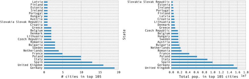
Figure 12-2. The number of cities in the list of the top 105 most populated cities in Europe (left) and the total population in those cities (right), grouped by state
Time Series
Time series are a common form of data in which a quantity is given, for example, at regularly or irregularly spaced timestamps, or for fixed or variable time spans (periods). In pandas, there are dedicated data structures for representing these types of data. Series and DataFrame can have both columns and indices with data types describing timestamps and time spans. When dealing with temporal data it is particularly useful to be able to index the data with time data types. Using pandas time-series indexers, DatetimeIndex and PeriodIndex, we can carry out many common date, time, period, and calendar operations, such as selecting time ranges, shifting and resampling of the data points in a time series.
To generate a sequence of dates that can be used as an index in a pandas Series or DataFrame objects, we can, for example, use the date_range function. It takes the starting point as a date and time string (or, alternatively, a datetime object from the Python standard library) as a first argument, and the number of elements in the range can be set using the periods keyword argument:
In [59]: pd.date_range("2015-1-1", periods=31)
Out[59]: <class 'pandas.tseries.index.DatetimeIndex'>
         [2015-01-01, ..., 2015-01-31]
         Length: 31, Freq: D, Timezone: None
To specify the frequency of the timestamps (which defaults to one day), we can use the freq keyword argument, and instead of using periods to specify the number of points, we can give both starting and ending points as date and time strings (or datetime objects) as first and second argument. For example, to generate hourly timestamps between 00:00 and 12:00 on 2015-01-01, we can use:
In [60]: pd.date_range("2015-1-1 00:00", "2015-1-1 12:00", freq="H")
Out[60]: <class 'pandas.tseries.index.DatetimeIndex'>
         [2015-01-01 00:00:00, ..., 2015-01-01 12:00:00]
         Length: 13, Freq: H, Timezone: None
The date_range function returns an instance of DatetimeIndex, which can be used, for example, as an index for a Series or DataFrame object:
In [61]: ts1 = pd.Series(np.arange(31), index=pd.date_range("2015-1-1", periods=31))
In [62]: ts1.head()
Out[62]: 2015-01-01    0
         2015-01-02    1
         2015-01-03    2
         2015-01-04    3
         2015-01-05    4
         Freq: D, dtype: int64
The elements of a DatetimeIndex object can, for example, be accessed using indexing with date and time strings. An element in a DatetimeIndex is of the type Timestamp, which is a pandas object that extends the standard Python datetime object (see the datetime module in the Python standard library).
In [63]: ts1["2015-1-3"]
Out[63]: 2
In [64]: ts1.index[2]
Out[64]: Timestamp('2015-01-03 00:00:00', offset='D')
In many aspects, a Timestamp and datetime object are interchangeable, and the Timestamp class have, like the datetime class, attributes for accessing time fields such as year, month, day, hour, minute, and so on. However, a notable difference between Timestamp and datetime is that Timestamp store a timestamp with nanoseconds resolution, while a datetime object only uses microsecond resolution.
In [65]: ts1.index[2].year, ts1.index[2].month, ts1.index[2].day
Out[65]: (2015, 1, 3)
In [66]: ts1.index[2].nanosecond
Out[66]: 0
We can convert a Timestamp object to a standard Python datetime object using the to_pydatetime method:
In [67]: ts1.index[2].to_pydatetime()
Out[67]: datetime.datetime(2015, 1, 3, 0, 0)
and we can use a list of datetime objects to create a pandas time series:
In [68]: import datetime
In [69]: ts2 = pd.Series(np.random.rand(2),
    ...:                 index=[datetime.datetime(2015, 1, 1), datetime.datetime(2015, 2, 1)])
In [70]: ts2
Out[70]: 2015-01-01    0.683801
         2015-02-01    0.916209
         dtype: float64
Data that is defined for sequences of time spans can be represented using Series and DataFrame objects that are indexed using the PeriodIndex class. We can construct an instance of the PeriodIndex class explicitly by passing a list of Period objects, and then specify it as an index when creating a Series or DataFrame object:
In [71]: periods = pd.PeriodIndex([pd.Period('2015-01'),
    ...:                           pd.Period('2015-02'),
    ...:                           pd.Period('2015-03')])
In [72]: ts3 = pd.Series(np.random.rand(3), index=periods)
In [73]: ts3
Out[73]: 2015-01    0.969817
         2015-02    0.086097
         2015-03    0.016567
         Freq: M, dtype: float64
In [74]: ts3.index
Out[74]: <class 'pandas.tseries.period.PeriodIndex'>
         [2015-01, ..., 2015-03]
         Length: 3, Freq: M
We can also converting a Series or DataFrame object indexed by a DatetimeIndex object to a PeriodIndex using the to_period method (which takes an argument that specifies the period frequency, here 'M' for month):
In [75]: ts2.to_period('M')
Out[75]: 2015-01    0.683801
         2015-02    0.916209
         Freq: M, dtype: float64
In the remaining part of this section we explore select features of pandas time series through examples. We look at the manipulation of two time series that contain sequences of temperature measurements at given timestamps. We have one dataset for an indoor temperature sensor, and one dataset for an outdoors temperature sensor, both with observations approximately every 10 minutes during most of 2014. The two data files, temperature_indoor_2014.tsv and temperature_outdoor_2014.tsv, are TSV (tab-separated values, a variant of the CSV format) files with two columns: the first column contains UNIX timestamps (seconds since Jan 1, 1970), and the second column is the measured temperature in degree Celsius. For example, the first five lines in the outdoor dataset are:
In [76]: !head -n 5 temperature_outdoor_2014.tsv
1388530986      4.380000
1388531586      4.250000
1388532187      4.190000
1388532787      4.060000
1388533388      4.060000
We can read the data files using read_csv by specifying that the delimiter between columns is the TAB character: delimiter=" ". When reading the two files we also explicitly specify the column names using the names keyword argument, since the files in this example do not have header lines with the column names.
In [77]: df1 = pd.read_csv('temperature_outdoor_2014.tsv', delimiter="	",
    ...:                   names=["time", "outdoor"])
In [78]: df2 = pd.read_csv('temperature_indoor_2014.tsv', delimiter="	",
    ...:                   names=["time", "indoor"])
Once we have created DataFrame objects for the time series data, it is informative to inspect the data by displaying the first few lines:

The next step toward a meaningful representation of the time series data is to convert the UNIX timestamps to date and time objects using to_datetime with the unit="s" argument. Furthermore, we localize the timestamps (assigning a time zone) using tz_localize and convert the time zone attribute to the Europe/Stockholm time zone using tz_convert. We also set the time column as index using set_index:

Displaying the first few rows of the data frame for the outdoor temperature dataset shows that the index now indeed is a date and time object. As we will see examples of in the following, having the index of a time series represented as proper date and time objects (in contrast to using for example integers representing the UNIX timestamps) allows us to easily perform many time-oriented operations. Before we proceed to explore the data in more detail, we first plot the two time series to obtain an idea of how the data looks like. For this we can use the DataFrame.plot method, and the results are shown in Figure 12-3. Note that there is data missing for a part of August. Imperfect data is a common problem, and handling missing data in a suitable manner is an important part of the mission statement of the pandas library.
In [85]: fig, ax = plt.subplots(1, 1, figsize=(12, 4))
    ...: df1.plot(ax=ax)
    ...: df2.plot(ax=ax)

Figure 12-3. Plot of the time series for indoors and outdoors temperatures
It is also illuminating to display the result of the info method of the DataFrame object. Doing so tells us that there are nearly 50000 data points in this data set, and that it contains data points starting at 2014-01-01 00:03:06 and ending at 2014-12-30 23:56:35:
In [86]: df1.info()
<class 'pandas.core.frame.DataFrame'>
DatetimeIndex: 49548 entries, 2014-01-01 00:03:06+01:00 to 2014-12-30 23:56:35+01:00
Data columns (total 1 columns):
outdoor    49548 non-null float64
dtypes: float64(1) memory usage: 774.2 KB
A common operation on time series is to select and extract parts of the data. For example, from the full dataset that contains data for all of 2014, we may be interested in selecting out and analyze only the data for the month of January. In pandas, we can accomplish this in a number of ways. For example, we can use Boolean indexing of a DataFrame to create a DataFrame for a subset of the data. To create the Boolean indexing mask that selects the data for January, we can take advantage of the pandas time series features that allows us to compare the time series index with string representations of a date and time. In the following code, the expressions like df1.index >= "2014-1-1," where df1.index is a time DateTimeIndex instance, results in a Boolean NumPy array that can be used as a mask to select the desired elements.
In [87]: mask_jan = (df1.index >= "2014-1-1") & (df1.index < "2014-2-1")
In [88]: df1_jan = df1[mask_jan]
In [89]: df1_jan.info()
<class 'pandas.core.frame.DataFrame'>
DatetimeIndex: 4452 entries, 2014-01-01 00:03:06+01:00 to 2014-01-31 23:56:58+01:00
Data columns (total 1 columns):
outdoor    4452 non-null float64
dtypes: float64(1) memory usage: 69.6 KB
Alternatively, we can use slice syntax directly with date and time strings:
In [90]: df2_jan = df2["2014-1-1":"2014-1-31"]
The results are two DataFrame objects, df1_jan and df2_jan, that contains data only for the month of January. Plotting this subset of the original data using the plot method results in the graph shown in Figure 12-4.
In [91]: fig, ax = plt.subplots(1, 1, figsize=(12, 4))
    ...: df1_jan.plot(ax=ax)
    ...: df2_jan.plot(ax=ax)

Figure 12-4. Plot of the time series for indoors and outdoors temperatures for a selected month (January)
Like the datetime class in Python’s standard library, the Timestamp class that is used in pandas to represent time values has attributes for accessing fields such as year, month, day, hour, minute, and so on. These fields are particularly useful when processing time series. For example, if we wish to calculate the average temperature for each month of the year, we can begin by creating a new column month, which we assign to the month field of the Timestamp values of the DatetimeIndex indexer. To extract the month field from each Timestamp value, we first call reset_index to convert the index to a column in the data frame (in which case the new DataFrame object falls back to using an integer index), after which we can use the apply function on the newly created time column.4

Next, we can group the DataFrame by the new month field, and aggregate the grouped values using the mean function for computing the average within each group.
In [95]: df1_month = df1_month.groupby("month").aggregate(np.mean)
In [96]: df2_month = df2.reset_index()
In [97]: df2_month["month"] = df2_month.time.apply(lambda x: x.month)
In [98]: df2_month = df2_month.groupby("month").aggregate(np.mean)
After having repeated the same process for the second DataFrame (indoor temperatures), we can combine df1_month and df2_month into a single DataFrame using the join method:

In only a few lines of code, we have here leveraged some of the many data processing capabilities of pandas to transform and compute with the data. It is often the case that there are many different ways to combine the tools provided by pandas to do the same, or a similar, analysis. For the current example, we can do the whole process in a single line of code, using the to_period and groupby methods, and the concat function (which like join combines DataFrame into a single DataFrame):

To visualize the results, we plot the average monthly temperatures as a bar plot and a box plot using the DataFrame method plot. The result is shown in Figure 12-5.
In [103]: fig, axes = plt.subplots(1, 2, figsize=(12, 4))
     ...: df_month.plot(kind='bar', ax=axes[0])
     ...: df_month.plot(kind='box', ax=axes[1])

Figure 12-5. Average indoor and outdoor temperatures per month (left), and a boxplot for monthly indoor and outdoors temperature (right)
Finally, a very useful feature of the pandas time series objects is the ability to up- and down-sample the time series using the resample method. Resampling means that the number of data points in a time series is changed. It can be either increased (upsampling) or decreased (downsampling). For upsampling, we need to choose a method for filling in the missing values, and for downsampling we need to choose a method for aggregating multiple sample points between each new sample point. The resample method expects as first argument a string that specifies the new period of data points in the resampled time series. For example, the string H represents a period of one hour, the string D one day, the string M one month, and so on.5 We can also combine these in simple expressions, such as 7D, which denotes a time period of seven days. Optionally, we can also use the how argument to specify how to aggregate values in the case of downsampling, and the fill_method argument to specify a method for filling in the value of new data points in the case of upsampling.
To illustrate the use for the resample method, consider the previous two time series with temperature data. The original sampling frequency is roughly 10 minutes, which amounts to a lot of data points over the period of a year. For plotting purposes, or if we want to compare the 2 time series, which are sampled at slightly different timestamps, it is often necessary to down-sample the original data. This can give less busy graphs, and regularly spaced time series that readily can be compared to each other. In the following code we resample the outdoors temperature time series to four different sampling frequencies, and plot the resulting time series. We also resample both the outdoor and indoor time series to daily averages that we subtract to obtain the daily average temperature difference between indoors and outdoors throughout the year. These types of manipulations are very handy when dealing time series, and it is one of the many areas in which the pandas library really shines. See Figure 12-6.
In [104]: df1_hour = df1.resample("H")
In [105]: df1_hour.columns = ["outdoor (hourly avg.)"]
In [106]: df1_day = df1.resample("D")
In [107]: df1_day.columns = ["outdoor (daily avg.)"]
In [108]: df1_week = df1.resample("7D")
In [109]: df1_week.columns = ["outdoor (weekly avg.)"]
In [110]: df1_month = df1.resample("M")
In [111]: df1_month.columns = ["outdoor (monthly avg.)"]
In [112]: df_diff = (df1.resample("D").outdoor - df2.resample("D").indoor)
In [113]: fig, (ax1, ax2) = plt.subplots(2, 1, figsize=(12, 6))
     ...: df1_hour.plot(ax=ax1, alpha=0.25)
     ...: df1_day.plot(ax=ax1)
     ...: df1_week.plot(ax=ax1)
     ...: df1_month.plot(ax=ax1)
     ...: df_diff.plot(ax=ax2)
     ...: ax2.set_title("temperature difference between outdoor and indoor")
     ...: fig.tight_layout()

Figure 12-6. Outdoors temperature, resampled to hourly, daily, weekly, and monthly averages
As an illustration of upsampling, consider the following example where we resample the data frame df1 to a sample frequency of 5 minutes, using three different fill methods (None, ffill for forward-fill, and bfill for back-fill). The original sample frequency is approximately 10 minutes, so this resampling is indeed upsampling. The result is three new data frames that we combine into a single DataFrame object using the concat function. The first five rows in the data frame are also shown below. Note that the every second data point is a new sample point, and depending on the value of the fill_method argument those values are filled (or not) according to the specified strategies. When no fill strategy is selected, the corresponding values are marked as missing using the NaN value.

The Seaborn Graphics Library
The seaborn graphics library is built on top of Matplotlib, and it provides functions for generating graphs that are useful when working with statistics and data analysis, including distribution plots, kernel-density plots, joint distribution plots, factor plot, heat maps, facet plots, and several ways of visualizing regressions. It also provides methods for coloring data in graphs, and numerous well-crafted color palettes. The seaborn library is created with close attention to the aesthetics of the graphs it produces, and the graphs generated with the library tend to be both good looking and informative. The seaborn library distinguishes itself from the underlying Matplotlib library in that it provides polished higher-level graph functions for a specific application domain, namely, statistical analysis and data visualization. The ease with which standard statistical graphs can be generated with the library makes it a valuable tool in exploratory data analysis.
To get started using the seaborn library, we first import the seaborn module. Here we follow the common convention of importing this library under the name sns. After importing the library we can set a style for the graphs it produces using the sns.set function. Here we choose to work with the style called darkgrid, which produces graphs with a gray background (also try the whitegrid style).
In [116]: import seaborn as sns
In [117]: sns.set(style="darkgrid")
Importing seaborn and setting a style for the library alters the default settings for how Matplotlib graphs appear, including graphs produced by the pandas library. For example, consider the following plot of the previously used indoor and outdoor temperature time series. The resulting graph is shown in Figure 12-7, and although the graph was produced using the pandas DataFrame method plot, importing the seaborn library has changed the appearance of the graph (compare with Figure 12-3).
In [118]: df1 = pd.read_csv('temperature_outdoor_2014.tsv', delimiter="	",
     ...:                   names=["time", "outdoor"])
     ...: df1.time = (pd.to_datetime(df1.time.values, unit="s")
     ...:               .tz_localize('UTC').tz_convert('Europe/Stockholm'))
     ...: df1 = df1.set_index("time").resample("10min")
In [119]: df2 = pd.read_csv('temperature_indoor_2014.tsv', delimiter="	",
     ...:                   names=["time", "indoor"])
     ...: df2.time = (pd.to_datetime(df2.time.values, unit="s")
     ...:               .tz_localize('UTC').tz_convert('Europe/Stockholm'))
     ...: df2 = df2.set_index("time").resample("10min")
In [120]: df_temp = pd.concat([df1, df2], axis=1)
In [121]: fig, ax = plt.subplots(1, 1, figsize=(8, 4))
     ...: df_temp.resample("D").plot(y=["outdoor", "indoor"], ax=ax)

Figure 12-7. Time series plot produced by Matplotlib using the pandas library, with a plot style that is set up by the seaborn library
The main strength of the seaborn library, apart from generating good-looking graphics, is its collection of easy-to-use statistical plots. Examples of these are the kdeplot and distplot, which plot a kernel-density estimate plot and a histogram plot with a kernel-density estimate overlaid on top of the histogram, respectively. For example, the following two lines of code produce the graph shown in Figure 12-8. The solid blue and green lines in this figure are the kernel-density estimate that can also be graphed separately using the function kdeplot (not shown here).
In [122]: sns.distplot(df_temp.to_period("M")["outdoor"]["2014-04"].dropna().values, bins=50);
     ...: sns.distplot(df_temp.to_period("M")["indoor"]["2014-04"].dropna().values, bins=50);

Figure 12-8. The histogram (bars) and kernel-density plots (solid lines) for the subset of the indoors and outdoors datasets that correspond to the month of april
The kdeplot function can also operate on two-dimensional data, showing a contour graph of the joint kernel-density estimate. Relatedly, we can use the jointplot function to plot the joint distribution for two separate datasets. Below we use the kdeplot and jointplot to show the correlation between the indoor and outdoor data series, which are resampled to hourly averages before visualized (we also drop missing values using dropna method, since the functions form the seaborn library do not accept arrays with missing data). The results are shown in Figure 12-9.
In [123]: sns.kdeplot(df_temp.resample("H")["outdoor"].dropna().values,
     ...:             df_temp.resample("H")["indoor"].dropna().values, shade=False)
In [124]: with sns.axes_style("white"):
     ...:     sns.jointplot(df_temp.resample("H")["outdoor"].values,
     ...:                   df_temp.resample("H")["indoor"].values, kind="hex")

Figure 12-9. Two-dimensional kernel-density estimate contours (left) and the joint distribution for the indoor and outdoor temperature datasets (right). The outdoor temperatures are shown on the x-axis, and the indoor temperature on the y-axis
The seaborn library also provides functions for working with categorical data. A simple example of a graph type that is often useful for datasets with categorical variables is the standard boxplot for visualizing the descriptive statistics (min, max, median, and quartiles) of a dataset. An interesting twist on the standard boxplot is violin plot, in which the kernel-density estimated is shown in the width of boxplot. The boxplot and violinplot functions can be used to produce such graphs, as shown in the following example, and the resulting graph is shown in Figure 12-10.
In [125]: fig, (ax1, ax2) = plt.subplots(1, 2, figsize=(8, 4))
     ...: sns.boxplot(df_temp.dropna(), ax=ax1, palette="pastel")
     ...: sns.violinplot(df_temp.dropna(), ax=ax2, palette="pastel")

Figure 12-10. A box plot (left) and violin plot (right) for the indoor and outdoor temperature datasets
As a further example of violin plots, consider the outdoor temperature dataset partitioned by the month, which can be produced by passing the month field of the index of the data frame as second argument (used to group the data into categories). The resulting graph, which is shown in Figure 12-11, provides a compact and informative visualization of the distribution of temperatures for each month of the year.
In [126]: sns.violinplot(x=df_temp.dropna().index.month,
     ...:                y=df_temp.dropna().outdoor, color="skyblue");

Figure 12-11. Violin plot for the outdoor temperature grouped by month
Heat maps are another type of graph that is handy when dealing with categorical variables, especially for variables with a large number of categories. The seaborn library provides the function heatmap for generating this type of graph. For example, working with the outdoors temperature data set, we can create two categorical columns month and hour by extracting those fields from the index and assign them to new columns in the data field. Next we can use the pivot_table function in pandas to pivot the columns into a table (matrix) where two selected categorical variables constitute the new index and columns. Here we pivot the temperature dataset so that the hours of the day are the columns, and the months of the year are the rows (index). To aggregate the multiple data points that falls within each hour-month category, we use aggfunc=np.mean argument to compute the mean of all the values:
In [127]: df_temp["month"] = df_temp.index.month
     ...: df_temp["hour"] = df_temp.index.hour
In [128]: table = pd.pivot_table(df_temp, values='outdoor', index=['month'],
     ...:                        columns=['hour'], aggfunc=np.mean)
Once we have created pivot table, we can visualize it as a heatmap using the heatmap function in seaborn. The result is shown in Figure 12-12.
In [129]: fig, ax = plt.subplots(1, 1, figsize=(8, 4))
     ...: sns.heatmap(table, ax=ax)

Figure 12-12. A heatmap of the outdoor temperature data grouped by hour of the day and month of the year
The seaborn library contains much more statistical visualization tools than what we have been able to survey here. However, I hope that looking at a few examples of what this library can do illustrates the essence of the seaborn library – that it is a convenient tool for statistical analysis and exploration of data, which is able to produce many standard statistical graphs with a minimal of effort. In the following chapters we will see further examples of applications of the seaborn library.
Summary
In this chapter we have explored data representation and data processing using the pandas library, and we briefly surveyed the statistical graphics tools provided by the seaborn visualization library. The pandas library provides the back end for much of data wrangling done with Python. It achieves this by adding a higher-level abstraction layer in the data representation on top of NumPy arrays, with additional methods for operating on the underlying data. The ease with which data can be loaded, transformed, and manipulated makes it an invaluable part of the data processing workflow in Python. The pandas library also contains basic functions for visualizing the data that is represented by its data structures. Being able to quickly visualize data represented as pandas series and data frames is an important tool in exploratory data analytics as well as for presentation. The seaborn library takes this a step further, and provides a rich collection of statistical graphs that can be produced often with a single line of code. Many functions in the seaborn library can operate directly on pandas data structures.
Further Reading
A great introduction to the pandas library is given by the original creator of the library in (McKinney, 2013), and it is also a rather detailed introduction to NumPy. The pandas official documentation, available at http://pandas.pydata.org/pandas-docs/stable, also provides an accessible and very detailed description of the features of the library. Another good online resource for learning pandas is http://github.com/jvns/pandas-cookbook. For data visualization, we have looked at the seaborn library in this chapter, and it is well described in the documentation available on its web site. With respect to higher-level visualization tools, it is also worth exploring the ggplot library for Python: http://ggplot.yhathq.com, which is an implementation based on renowned Grammar of graphics (L. Wilkinson, 2005). This library is also closely integrated with the pandas library, and it provides statistical visualization tools that are convenient when analyzing data. For more information about visualization in Python, see for example, the book by Vaingast.
References
McKinney, W. (2013). Python for Data Analysis. Sebastopol: O’Reilly.
Vaingast, S. (2014). Beginning Python Visualization. New York: Apress.
L. Wilkinson, D. W. (2005). The Grammar of Graphics. Chicago: Springer.
_________________
1Also known as data munging or data wrangling.
2CSV, or comma-separated values, is a common text format where rows are stored in lines and columns are separated by a comma (or some other text delimiter). See Chapter 18 for more details about this and other file formats.
3This dataset was obtained from the Wiki page: http://en.wikipedia.org/wiki/Largest_cities_of_the_European_Union_by_population_within_city_limits.
4We can also directly use the month method of the DatetimeIndex index object, but for the sake of demonstration we use a more explicit approach here.
5There are a large number of available time-unit codes. See the sections on “Offset aliases” and “Anchored offsets” in the pandas reference manual for details.