
![]()
Partial Differential Equations
Partial differential equations (PDEs) are multivariate different equations where derivatives of more than one dependent variable occur. That is, the derivatives in the equation are partial derivatives. As such they are generalizations of ordinary differentials equations, which were covered in Chapter 9. Conceptually, the difference between ordinary and partial differential equations is not that big, but the computational techniques required to deal with ODEs and PDEs are very different, and solving PDEs is typically much more computationally demanding. Most techniques for solving PDEs numerically are based on the idea of discretizing the problem in each independent variable that occurs in the PDE, and thereby recasting the problem into an algebraic form. This usually results in very large-scale linear algebra problems. Two common techniques for recasting PDEs into algebraic form is the finite-difference methods (FDMs), where the derivatives in the problem are approximated with their finite-difference formula; and the finite-element methods (FEMs), where the unknown function is written as linear combination of simple basis functions that can be differentiated and integrated easily. The unknown function is described by a set of coefficients for the basis functions in this representation, and by a suitable rewriting of the PDEs we can obtain algebraic equations for these coefficients.
With both FDMs and FEMs, the resulting algebraic equation system is usually very large, and in matrix form such equation systems are usually very sparse. Both FDM and FEM therefore heavily rely on sparse matrix representation for the algebraic linear equations, as discussed in Chapter 10. Most general-purpose frameworks for PDEs are based on FEM, or some variant thereof, as this method allows for solving very general problems on complicated problem domains.
Solving PDE problems can be far more resource demanding compared to other types of computational problems that we have covered so far (for example, compared to ODEs). It can be resource demanding partly because the number of points required to discretize a region of space scale exponentially with the number of dimensions. If a one-dimensional problem requires 100 points to describe, a two-dimensional problem with similar resolution requires ![]() points, and a three-dimensional problem requires
points, and a three-dimensional problem requires ![]() points. Since each point in the discretized space corresponds to an unknown variable, it is easy to imagine that PDE problems can result in very large equation systems. Defining PDE problems programmatically can also be complicated. One reason for this is that the possible forms of a PDE vastly outnumber the more limited possible forms of ODEs. Another reason is geometry: while an interval in one-dimensional space is uniquely defined by two points, an area in two-dimensional problems and a volume in three-dimensional problems can have arbitrarily complicated geometries enclosed by curves and surfaces. To define the problem domain of a PDE and its discretization in a mesh of coordinate points can therefore require advanced tools, and there is a large amount of freedom in how boundary conditions can be defined as well. In contrast to ODE problems, there is no standard form on which any PDE problem can be defined.
points. Since each point in the discretized space corresponds to an unknown variable, it is easy to imagine that PDE problems can result in very large equation systems. Defining PDE problems programmatically can also be complicated. One reason for this is that the possible forms of a PDE vastly outnumber the more limited possible forms of ODEs. Another reason is geometry: while an interval in one-dimensional space is uniquely defined by two points, an area in two-dimensional problems and a volume in three-dimensional problems can have arbitrarily complicated geometries enclosed by curves and surfaces. To define the problem domain of a PDE and its discretization in a mesh of coordinate points can therefore require advanced tools, and there is a large amount of freedom in how boundary conditions can be defined as well. In contrast to ODE problems, there is no standard form on which any PDE problem can be defined.
For these reasons, the PDE solvers for Python are only available through libraries and frameworks that are specifically dedicated to PDE problems. For Python, there are at least three significant libraries for solving PDE problems using the FEM method: the FiPy library, the SfePy library, and the FEniCS library. All of these libraries are extensive and feature rich, and going into the details of using either of these libraries is beyond the scope of this book. Here we can only give a brief introduction to PDE problems and survey prominent examples of PDE libraries that can be used from Python, and go through a few examples that illustrate some of the features of one of these libraries (FEniCS). The hope is that this can give the reader who is interested in solving PDE problems with Python a birds-eye overview of the available options, and some useful pointers to where to look for further information.
Importing Modules
For basic numerical and plotting usage, in this chapter too we require the NumPy and Matplotlib libraries. For 3D plotting we need to explicitly import the mplot3d module from the Matplotlib toolkit library mpl_toolkits. As usual we assume that these libraries are imported in the following manner:
In [1]: import numpy as np
In [2]: import matplotlib.pyplot as plt
In [3]: import matplotlib as mpl
In [4]: import mpl_toolkits.mplot3d
We also use the linalg and the sparse modules from SciPy, and to use the linalg sub module of the sparse module, we also need to import it explicitly:
In [5]: import scipy.sparse as sp
In [6]: import scipy.sparse.linalg
In [7]: import scipy.linalg as la
With these imports, we can access the dense linear algebra module as la, while the sparse linear algebra module is accessed as sp.linalg. Furthermore, later in this chapter we will also use the FEniCS FEM framework, and we require that its dolfin and mshr libraries be imported in the following manner:
In [8]: import dolfin
In [9]: import mshr
Partial Differential Equations
The unknown quantity in a PDE is a multivariate function, here denoted as u. In an n-dimensional problem, the function u depends on n independent variables: u(x1, x2, ..., xn). A general PDE can formally be written as

where  denotes all first-order derivatives with respect to the independent variables x1, ..., xn,
 denotes all second-order derivatives, and so on. Here F is a known function that describes the form of the PDE, and Ω is the domain of the PDE problem. Many PDEs that occur in practice only contain up to second-order derivatives, and we typically deal with problems in two or three spatial dimensions, and possibly time. When working with PDEs, it is common to simplify the notation by denoting the partial derivatives with respect to an independent variable x using the subscript notation:
 ![]() . Higher-order derivatives are denoted with multiple indices:
. Higher-order derivatives are denoted with multiple indices: ![]() ,
, ![]() , and so on. An example of a typical PDE is the heat equation, which in a two-dimensional Cartesian coordinate system takes the form
, and so on. An example of a typical PDE is the heat equation, which in a two-dimensional Cartesian coordinate system takes the form ![]() . Here the function
. Here the function ![]() describes the temperature at the spatial point (x, y) at time t, and α is the thermal diffusivity coefficient.
describes the temperature at the spatial point (x, y) at time t, and α is the thermal diffusivity coefficient.
To fully specify a particular solution to a PDE, we need to define its boundary conditions, which are known values of the function or a combination of its derivatives along the boundary of the problem domain Ω, as well as the initial values if the problem is time dependent. The boundary is often denoted as Γ or ![]() and in general different boundary conditions can be given for different parts of the boundary. Two important types of boundary conditions are Dirichlet boundary conditions, which specifies the value of the function at the boundary,
and in general different boundary conditions can be given for different parts of the boundary. Two important types of boundary conditions are Dirichlet boundary conditions, which specifies the value of the function at the boundary, ![]() for
for ![]() ; and Neumann boundary conditions, which specifies the normal derivative on the boundary,
; and Neumann boundary conditions, which specifies the normal derivative on the boundary, ![]() for
for ![]() where the n is the outward normal from the boundary. Here g(x) and h(x) are arbitrary functions.
where the n is the outward normal from the boundary. Here g(x) and h(x) are arbitrary functions.
Finite-Difference Methods
The basic idea of the finite-difference method is to approximate the derivatives that occur in a PDE with their finite-difference formulas on a discretized space. For example, the finite-difference formula for the ordinary derivative ![]() on a discretization of the continuous variable x into discrete points {xn} can be approximated with the forward difference formula
on a discretization of the continuous variable x into discrete points {xn} can be approximated with the forward difference formula ![]() , the backward difference formula
, the backward difference formula ![]() or the centered difference formula
or the centered difference formula ![]() Similarly, we can also construct finite-difference formulas for higher-order derivatives, such as the second-order derivative
Similarly, we can also construct finite-difference formulas for higher-order derivatives, such as the second-order derivative  Assuming that the discretization of the continuous variable x into discrete points is fine enough, these finite-difference formulas can give good approximations of the derivatives. Replacing derivatives in an ODE or PDE with their finite-difference formulas recasts the equations from differential equations to algebraic equations. If the original ODE or PDE is linear, the algebraic equations are also linear, and can be solved with standard linear algebra methods.
To make this method more concrete, consider the ODE problem ![]() in the interval
in the interval ![]() and with boundary conditions
and with boundary conditions ![]() and
and ![]() , which, for example, arises from the steady-state heat equation in one dimension. In contrast the ODE initial-value problem considered in Chapter 9, this is a boundary-value problem because the value of u is specified at both
, which, for example, arises from the steady-state heat equation in one dimension. In contrast the ODE initial-value problem considered in Chapter 9, this is a boundary-value problem because the value of u is specified at both ![]() and
and ![]() The methods for initial-value problems are therefore not applicable here. Instead we can treat this problem by dividing the interval [0, 1] into discrete points xn, and the problem is then to find the function
The methods for initial-value problems are therefore not applicable here. Instead we can treat this problem by dividing the interval [0, 1] into discrete points xn, and the problem is then to find the function ![]() at these points. Writing the ODE problem in finite-difference form gives an equation
at these points. Writing the ODE problem in finite-difference form gives an equation ![]() for every interior point n, with the boundary conditions
for every interior point n, with the boundary conditions ![]() and
and ![]() . Here the interval [0, 1] is discretized into
. Here the interval [0, 1] is discretized into ![]() evenly spaced points, including the boundary points, with separation
evenly spaced points, including the boundary points, with separation ![]() Since the function is known at the two boundary points, there are N unknown variables un corresponding to the function values at the interior points. The set of equations for the interior points can be written in a matrix form as
Since the function is known at the two boundary points, there are N unknown variables un corresponding to the function values at the interior points. The set of equations for the interior points can be written in a matrix form as ![]() where
where ![]() ,
,  and
and

Here the matrix A is describes the coupling of the equations for un to values at neighboring points due to the finite-difference formula that was used to approximate the second-order derivative in the ODE. The boundary values are included in the b vector, which also contains the constant right-hand side of the original ODE (the source term). At this point we can straightforwardly solve the linear equation system ![]() for the unknown vector of u and thereby obtain the approximate values of the function u(x) at the discete points {xn}.
for the unknown vector of u and thereby obtain the approximate values of the function u(x) at the discete points {xn}.
In Python code, we can set up and solve this problem in the following way: First, we define variables for the number of interior points N, the values of the function at the boundaries u0 and u1, as well as the spacing between neighboring points dx.
In [10]: N = 5
In [11]: u0, u1 = 1, 2
In [12]: dx = 1.0 / (N + 1)
Next we construct the matrix A as described above. For this we can use the eye function in NumPy, which creates two-dimensional arrays with ones on the diagonal, or on the upper or lower diagonal that are shifted from the main diagonal by the number given by the argument k.
In [13]: A = (np.eye(N, k=-1) - 2 * np.eye(N) + np.eye(N, k=1)) / dx**2
In [14]: A
Out[14]: array([[-72.,  36.,   0.,   0.,   0.],
                [ 36., -72.,  36.,   0.,   0.],
                [  0.,  36., -72.,  36.,   0.],
                [  0.,   0.,  36., -72.,  36.],
                [  0.,   0.,   0.,  36., -72.]])
Next we need to define an array for the vector b, which corresponds to the source term -5 in the differential equation, as well as the boundary condition. The boundary conditions enters into the equations via the finite-difference expressions for the derivatives of the first and the last equation (for u1 and uN), but these terms are missing from the expression represented by the matrix A, and must therefore be added to the vector b.
In [15]: b = -5 * np.ones(N)
    ...: b[0] -= u0 / dx**2
    ...: b[N-1] -= u1 / dx**2
Once the matrix A and the vector b are defined, we can proceed to solve the equation system using the linear equation solver from SciPy (we could also use the one provided by NumPy, np.linalg.solve).
In [16]: u = la.solve(A, b)
This completes the solution of this ODE problem. To visualize the solution, here we first create an array x that contains the discrete coordinate points for which we have solved the problem, including the boundary points, and we also create an array U that combines the boundary values and the interior points in one array. The result is then plotted and shown in Figure 11-1.
In [17]: x = np.linspace(0, 1, N+2)
In [18]: U = np.hstack([[u0], u, [u1]])
In [19]: fig, ax = plt.subplots(figsize=(8, 4))
    ...: ax.plot(x, U)
    ...: ax.plot(x[1:-1], u, 'ks')
    ...: ax.set_xlim(0, 1)
    ...: ax.set_xlabel(r"$x$", fontsize=18)
    ...: ax.set_ylabel(r"$u(x)$", fontsize=18)

Figure 11-1. Solution to the second-order ODE boundary-value problem introduced in the text
The finite-difference method can easily be extended to higher dimensions by using the finite-difference formula along each discretized coordinate. For a two-dimensional problem, we have a two-dimensional array u for the unknown interior function values, and when using the finite differential formula we obtain a system of coupled equations for the elements in u. To write these equations on the standard matrix-vector form, we can rearrange the u array into a vector, and assemble the corresponding matrix A from the finite-difference equations.
As an example, consider the following two-dimensional generalization of the previous problem: ![]() , with the boundary conditions
, with the boundary conditions ![]() ,
, ![]() ,
, ![]() , and
, and ![]() . Here there is no source term, but the boundary conditions in a two-dimensional problem are more complicated than in the one-dimensional problem we solved earlier. In finite-difference form, we can write the PDE as
. Here there is no source term, but the boundary conditions in a two-dimensional problem are more complicated than in the one-dimensional problem we solved earlier. In finite-difference form, we can write the PDE as ![]() . If we divide the x and y intervals into N interior points (
. If we divide the x and y intervals into N interior points (![]() points including the boundary points), then
points including the boundary points), then ![]() and u is a NxN matrix. To write the equation on the standard form
and u is a NxN matrix. To write the equation on the standard form ![]() , we can rearrange the matrix u by stacking its rows or columns into a vector of size
, we can rearrange the matrix u by stacking its rows or columns into a vector of size ![]() . The matrix A is then of size
. The matrix A is then of size ![]() which can be very big if we need to use a fine discretization of the x and y coordinates. For example, using 100 points along both x and y gives an equation system that has 104 unknown values umn, and the matrix A has
which can be very big if we need to use a fine discretization of the x and y coordinates. For example, using 100 points along both x and y gives an equation system that has 104 unknown values umn, and the matrix A has ![]() elements. Fortunately, since the finite-difference formula only couples neighboring points, the matrix A turns out to be very sparse, and here we can benefit greatly from working with sparse matrices, as we will see in the following.
elements. Fortunately, since the finite-difference formula only couples neighboring points, the matrix A turns out to be very sparse, and here we can benefit greatly from working with sparse matrices, as we will see in the following.
To solve this PDE problem with Python and the finite-element method, we start by defining variables for the number of interior points and the values along the four boundaries of the unit square:
In [20]: N = 100
In [21]: u0_t, u0_b = 5, -5
In [22]: u0_l, u0_r = 3, -1
In [23]: dx = 1. / (N+1)
We also computed the separation dx between the uniformly spaced coordinate points in the discretization of x and y (assumed equal). Because the finite-difference formula couples both neighboring rows and columns, it is slightly more involved to construct the matrix A for this example. However, a relatively direct approach is to first define the matrix A_1d that corresponds to the one-dimensional formula along one of the coordinates (say x, or the index m in um,n). To distribute this formula along each row, we can take the tensor product of the identity matrix of size ![]() with the A_1d matrix. The result describes all derivatives along the m-index for all values indices n. To cover the terms that couple the equation for um,n to
with the A_1d matrix. The result describes all derivatives along the m-index for all values indices n. To cover the terms that couple the equation for um,n to ![]() and
and ![]() that is the derivatives along the index n, we need to add diagonals that are separated from the main diagonal by N positions. In the following we perform these steps to construct A using the eye and kron functions from the scipy.sparse module. The result is a sparse matrix A that describes the finite-difference equation system for the two-dimensional PDE we are considering here:
that is the derivatives along the index n, we need to add diagonals that are separated from the main diagonal by N positions. In the following we perform these steps to construct A using the eye and kron functions from the scipy.sparse module. The result is a sparse matrix A that describes the finite-difference equation system for the two-dimensional PDE we are considering here:
In [24]: A_1d = (sp.eye(N, k=-1) + sp.eye(N, k=1) - 4 * sp.eye(N))/dx**2
In [25]: A = sp.kron(sp.eye(N), A_1d) + (sp.eye(N**2, k=-N) + sp.eye(N**2, k=N))/dx**2
In [26]: A
Out[26]: <10000x10000 sparse matrix of type '<type 'numpy.float64'>'
                 with 49600 stored elements in Compressed Sparse Row format>
The printout of A shows that it is a sparse matrix with 108 elements with 49600 nonzero elements, so that only one out of about 2000 elements is nonzero, and A is indeed very sparse. To construct the vector b from the boundary conditions, it is convenient to create a ![]() array of zeros, and assign the boundary condition to edge elements of this array (which are the corresponding elements in u that are coupled to the boundaries, that is, the interior points that are neighbors to the boundary). Once this
array of zeros, and assign the boundary condition to edge elements of this array (which are the corresponding elements in u that are coupled to the boundaries, that is, the interior points that are neighbors to the boundary). Once this ![]() array is created and assigned, we can use the reshape method to rearrange it into a
array is created and assigned, we can use the reshape method to rearrange it into a ![]() vector that can be used in the
vector that can be used in the ![]() equation:
equation:
In [27]: b = np.zeros((N, N))
    ...: b[0, :] += u0_b   # bottom
    ...: b[-1, :] += u0_t  # top
    ...: b[:, 0] += u0_l   # left
    ...: b[:, -1] += u0_r  # right
    ...: b = - b.reshape(N**2) / dx**2
When the A and b arrays are created, we can proceed to solve the equation system for the vector v, and use the reshape method to arrange it back into the ![]() matrix u:
matrix u:
In [28]: v = sp.linalg.spsolve(A, b)
In [29]: u = v.reshape(N, N)
For plotting purposes, we also create a matrix U that combines the u matrix with the boundary conditions. Together with the coordinate matrices X and Y, we then plot a color map graph and a 3D surface view of the solution. The result is shown in Figure 11-2.
In [30]: U = np.vstack([np.ones((1, N+2)) * u0_b,
    ...:                np.hstack([np.ones((N, 1)) * u0_l, u, np.ones((N, 1)) * u0_r]),
    ...:                np.ones((1, N+2)) * u0_t])
In [31]: x = np.linspace(0, 1, N+2)
In [32]: X, Y = np.meshgrid(x, x)
In [33]: fig = plt.figure(figsize=(12, 5.5))
    ...: cmap = mpl.cm.get_cmap('RdBu_r')
    ...:
    ...: ax = fig.add_subplot(1, 2, 1)
    ...: c = ax.pcolor(X, Y, U, vmin=-5, vmax=5, cmap=cmap)
    ...: ax.set_xlabel(r"$x_1$", fontsize=18)
    ...: ax.set_ylabel(r"$x_2$", fontsize=18)
    ...:
    ...: ax = fig.add_subplot(1, 2, 2, projection='3d')
    ...: p = ax.plot_surface(X, Y, U, vmin=-5, vmax=5, rstride=3, cstride=3,
    ...:                     linewidth=0, cmap=cmap)
    ...: ax.set_xlabel(r"$x_1$", fontsize=18)
    ...: ax.set_ylabel(r"$x_2$", fontsize=18)
    ...: cb = plt.colorbar(p, ax=ax, shrink=0.75)
    ...: cb.set_label(r"$u(x_1, x_2)$", fontsize=18)
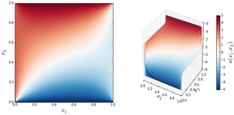
Figure 11-2. The solution to the two-dimensional heat equation with Dirichlet boundary conditions defined in the text
As mentioned above, FDM methods result in matrices A that are very sparse, and using sparse matrix data structures, such as those provided by scipy.sparse, can give significant performance improvements compared to using dense NumPy arrays. To illustrate in concrete terms the importance of using sparse matrices for this type of problems, we can compare the time required for solving of the ![]() equation using the IPython command %timeit, for the two cases where A is a sparse and a dense matrix:
equation using the IPython command %timeit, for the two cases where A is a sparse and a dense matrix:
In [34]: A_dense = A.todense()
In [35]: %timeit la.solve(A_dense, b)
1 loops, best of 3: 10.8 s per loop
In [36]: %timeit sp.linalg.spsolve(A, b)
10 loops, best of 3: 31.9 ms per loop
From these results, we see that using sparse matrices for the present problem results in a speedup of several orders of magnitude (in this particular case we have a speedup of a factor ![]() ).
).
The finite-difference method that we used in the last two examples is powerful and relatively simple method for solving ODE boundary-value problems and PDE problems with simple geometries. However, it is not so easily adapted to problems on more complicate domains, or problems on nonuniform coordinate grids. For such problems finite-element methods are typically more flexible and convenient to work with, and although FEMs are conceptually more complicated than FDMs, they can be computationally efficient and adapts well to complicated problem domains and more involved boundary conditions.
Finite-Element Methods
The Finite-Element Method (FEM) is powerful and universal method for converting PDEs into algebraic equations. The basic idea of this method is to represent the domain on which the PDE is defined with a finite set of discrete regions, or elements, and to approximate the unknown function as a linear combination of basis functions with local support on each of these elements (or on a small group of neighboring elements). Mathematically, this approximation solution, uh, represents a projection of the exact solution u in the function space V (for example, continuous real-valued functions) onto a finite subspace ![]() that is related to the discretization of the problem domain. If Vh is a suitable subspace of V, then it can be expected that uh can be a good approximation to u.
that is related to the discretization of the problem domain. If Vh is a suitable subspace of V, then it can be expected that uh can be a good approximation to u.
To be able to solve the approximate problem on the simplified function space Vh, we can first rewrite the PDE from its original formulation, which is known as the strong form, to its corresponding variational form, also known as the weak form. To obtain the weak form we multiply the PDE with an arbitrary function v and integrate over the entire problem domain. The function v is called a test function, and it can in general be defined on function space ![]() that differs from that of uh, which in this context is called a trial function.
that differs from that of uh, which in this context is called a trial function.
For example, consider the steady-state heat equation (also known as the Poisson equation) that we solved using the FDM earlier in this chapter: The strong form of this equation is ![]() , where we have used the vector operator notation. By multiplying this equation with a test function v and integrating over the domain
, where we have used the vector operator notation. By multiplying this equation with a test function v and integrating over the domain ![]() we obtain the weak form:
we obtain the weak form:
![]()
Since the exact solution u satisfies the strong form, it also satisfies the weak form of the PDE for any reasonable choice of v. The reverse does not necessarily hold true, but if a function uh satisfies the weak form for a large class of suitably chosen test functions v, then it is plausible that it is a good approximation to the exact solution u (hence the name test function).
To treat this problem numerically, we first need to make the transition from the infinite-dimensional function spaces V and ![]() to approximate finite-dimensional function spaces Vh and
to approximate finite-dimensional function spaces Vh and ![]() :
:
![]()
where ![]() and
and ![]() The key point here is that Vh and
The key point here is that Vh and ![]() are finite dimensional, so we can use a finite set of basis functions {øi} and
are finite dimensional, so we can use a finite set of basis functions {øi} and ![]() that spans the function spaces Vh and
that spans the function spaces Vh and ![]() respectively, to describe the functions uh and vh. In particular, we can express uk as a linear combination of the basis functions that spans its function space,
respectively, to describe the functions uh and vh. In particular, we can express uk as a linear combination of the basis functions that spans its function space, ![]() . Inserting this linear combination in the weak form of the PDE and carrying out the integrals and differential operators on the basis functions, instead of directly over terms in the PDE, yields a set of algebraic equations.
. Inserting this linear combination in the weak form of the PDE and carrying out the integrals and differential operators on the basis functions, instead of directly over terms in the PDE, yields a set of algebraic equations.
To obtain an equation system on the simple form ![]() , we also must write the weak form of the PDE on bilinear form with respect to the uh and vh functions:
, we also must write the weak form of the PDE on bilinear form with respect to the uh and vh functions: ![]() , for some functions a and L. This is not always possible, but for the current example of the Poission equation we can obtain this form by integrating by parts:
, for some functions a and L. This is not always possible, but for the current example of the Poission equation we can obtain this form by integrating by parts:
![]()
where in the second equality we have also applied Gauss theorem to convert the second term to an integral over the boundary ![]() of the domain Ω. Here n is the outward normal vector of the boundary
of the domain Ω. Here n is the outward normal vector of the boundary ![]() . There is no general method for rewriting a PDE on strong form to weak form, and each problem will have to be approached on a case-by-case basis. However, the technique used here, to integrate by part and rewrite the resulting integrals using integral identities, can be used for many frequently occurring PDEs.
. There is no general method for rewriting a PDE on strong form to weak form, and each problem will have to be approached on a case-by-case basis. However, the technique used here, to integrate by part and rewrite the resulting integrals using integral identities, can be used for many frequently occurring PDEs.
To reach the bilinear form that can be approached with standard linear algebra methods, we also have to deal with the boundary term in the weak form equation above. To this end, assume that the problem satisfies the Dirichlet boundary condition on a part of ![]() denoted ΓD, and Neumann boundary conditions on the remaining part of
denoted ΓD, and Neumann boundary conditions on the remaining part of ![]() , denoted ΓN:
, denoted ΓN: ![]() and
and ![]() Not all boundary conditions are of Dirichlet or Neumann type, but together these cover many physically motivated situation.
Not all boundary conditions are of Dirichlet or Neumann type, but together these cover many physically motivated situation.
Since we are free to choose the test functions vh, we can let vh vanish on the part of the boundary that satisfies Dirichlet boundary conditions. In this case we obtain the following weak form of the PDE problem:
![]()
If we substitute the function uk for its expression as a linear combination of basis functions, and substitute the test function with one of its basis functions, we obtain an algebraic equation:
![]()
If there are N basis functions in ![]() , then there are N unknown coefficients Ui, and we need N independent test functions
, then there are N unknown coefficients Ui, and we need N independent test functions ![]() to obtain a closed equation system. This equation system is on the form
to obtain a closed equation system. This equation system is on the form ![]() with
with
![]() and
and ![]() . Following this procedure we have therefore converted the PDE problem into a system of linear equations that can be readily solved.
. Following this procedure we have therefore converted the PDE problem into a system of linear equations that can be readily solved.
In practice, a very large number of basis functions can be required to obtain a good approximation to the exact solution, and the linear equation systems generated by FEMs are therefore often very large. However, the fact that each basis functions have support only at one or a few nearby elements in the discretization of the problem domain ensures that the matrix A is sparse, which makes it tractable to solve rather large-scale FEM problems. We also note that an important property of the basis functions øi and ![]() is that it should be easy to compute the derivatives and integrals of the expression that occur in the final weak form of the problem, so that the matrix A and vector b can be assembled efficiently. Typical examples of basis functions are low-order polynomial functions that are nonzero only within a single element. See Figure 11-3 for a one-dimensional illustration of this type of basis function, where the interval [0, 6] is discretized using five interior points, and a continuous function (black solid curve) is approximated as a piecewise linear function (dashed red line) by suitably weighted triangular basic functions (blue solid lines).
is that it should be easy to compute the derivatives and integrals of the expression that occur in the final weak form of the problem, so that the matrix A and vector b can be assembled efficiently. Typical examples of basis functions are low-order polynomial functions that are nonzero only within a single element. See Figure 11-3 for a one-dimensional illustration of this type of basis function, where the interval [0, 6] is discretized using five interior points, and a continuous function (black solid curve) is approximated as a piecewise linear function (dashed red line) by suitably weighted triangular basic functions (blue solid lines).

Figure 11-3. An example of possible basis functions (blue lines), with local support, for the one-dimensional domain [0, 6]
When using FEM software for solving PDE problems, it is typically required to convert the PDE to weak form by hand, and if possible rewrite it on the bilinear form ![]() . It is also necessary to provide a suitable discretization of the problem domain. This discretization is called a mesh, and it is usually made up of triangular partitioning (or their higher-order generalizations) of the total domain. Meshing an intricate problem domain can in itself be a complicated process, and it may require using sophisticated software especially dedicated for mesh generation. For simple geometries there are tools for programmatically generating meshes, and we will see examples of this in the following section.
. It is also necessary to provide a suitable discretization of the problem domain. This discretization is called a mesh, and it is usually made up of triangular partitioning (or their higher-order generalizations) of the total domain. Meshing an intricate problem domain can in itself be a complicated process, and it may require using sophisticated software especially dedicated for mesh generation. For simple geometries there are tools for programmatically generating meshes, and we will see examples of this in the following section.
Once a mesh is generated and the PDE problem is written on a suitable weak form, we can feed the problem into a FEM framework, which then automatically assembles the algebraic equation system and applies suitable sparse equation solvers to find the solution. In this processes, we often have a choice of what type of basis functions to use, as well as which type of solver to use. Once the algebraic equation is solved, we can construct the approximation solution to the PDE with the help of the basis functions, and we can for example visualize the solution or post process it in some other fashion.
In summary, solving a PDE using FEM typically involves the following steps:
- Generate a Mesh for the problem domain.
- Write the PDE on weak form.
- Program the problem in the FEM framework.
- Solve the resulting algebraic equations.
- Post process and/or visualize the solution.
In the following section we will review available FEM frameworks that can be used with Python, and then look at a number of examples that illustrates some of the key steps in the PDE solution process using FEM.
Survey of FEM Libraries
For Python there are at least three significant FEM packages: FiPy, SfePy, and FEniCS. These are all rather full-featured frameworks, which are capable of solving a wide range of PDE problems. Technically, the FiPy library is not a FEM software, but rather a finite-volume method (FVM) software, but the gist of this method is quite similar to FEM. The FiPy framework can be obtained from http://www.ctcms.nist.gov/fipy. The SfePy library is a FEM software that takes a slightly different approach to defining PDE problems, in that it uses Python files as configuration files for its FEM solver, rather programmatically setting up a FEM problem (although this mode of operation is technically also supported in SfePy). The SfePy library is available from http://sfepy.org. The third major framework for FEM with Python is FEniCS, which is written for C++ and Python. The FEniCS framework is my personal favorite when it comes to FEM software for Python, as it provides an elegant Python interface to a powerful FEM engine. Like FDM problem, FEM problems typically result in very large-scale equation systems that require using sparse matrix techniques to solve efficiently. A crucial part of a FEM framework is therefore to efficiently solve large-scale linear and nonlinear systems, using sparse matrices representation and direct or iterative solvers that work on sparse systems, possibly using parallelization. Each of the frameworks mentioned above supports multiple back ends for such low-level computations. For example, many FEM frameworks can use the PETSc and Trilinos frameworks.
Unfortunately we are not able to explore in depth how to use either of these FEM frameworks here, but in the following section we will look at solving example problems with FEniCS, and thereby introduce some of its basic features and usage. The hope is that the examples can give a flavor of how it is to work with FEM problems in Python, and provide a starting point for the readers interested in learning more about FEM with Python.
Solving PDEs using FEniCS
In this section we solve a series of increasingly complicated PDEs using the FEniCS framework, and in the process we introduce the workflow and a few of the main features of this FEM software. For a thorough introduction to the FEniCS framework, see the documentation at the project web sites and the official FEniCS book (Anders Logg, 2012).
![]() FEniCS FEniCS is a highly capable FEM framework that is made up of a collection of libraries and tools for solving PDE problem. Much of FEniCS is programmed in C++, but it also provides an official Python interface. Because of the complexity of the many dependencies of the FEniCS libraries to external low-level numerical libraries, FEniCS is usually packaged and installed as an independent environment. For more information about the FEniCS, see the project’s web site at http://fenicsproject.org. At the time of writing, the most recent version is 1.5.0.
FEniCS FEniCS is a highly capable FEM framework that is made up of a collection of libraries and tools for solving PDE problem. Much of FEniCS is programmed in C++, but it also provides an official Python interface. Because of the complexity of the many dependencies of the FEniCS libraries to external low-level numerical libraries, FEniCS is usually packaged and installed as an independent environment. For more information about the FEniCS, see the project’s web site at http://fenicsproject.org. At the time of writing, the most recent version is 1.5.0.
The Python interface to FEniCS is provided by a library named dolfin. For mesh generation we will also use the mshr library. In the following code, we assume that these libraries are imported in their entirety, as shown in the beginning of this chapter. For a summary of the most important functions and classes from these libraries, see Table 11-1 and Table 11-2.
Table 11-1. Summary of selected functions and classes in the dolfin library
|
Function/Class |
Description |
Example |
|---|---|---|
|
parameters |
Dictionary holding configuration parameters for the FEniCS framework. |
dolfin.parameters["reorder_dofs_serial"] |
|
RectangleMesh |
Object for generating a rectangular 2D mesh. |
mesh = dolfin.RectangularMesh(0, 0, 1, 1, 10, 10) |
|
MeshFunction |
Function defined over a given mesh. |
dolfin.MeshFunction("size_t", mesh, mesh.topology().dim()-1) |
|
FunctionSpace |
Object for representing a function space. |
V = dolfin.FunctionSpace(mesh, 'Lagrange', 1) |
|
TrialFunction |
Object for representing a trial function defined in a given function space. |
u = dolfin.TrialFunction(V) |
|
TestFunction |
Object for representing a test function defined in a given function space. |
v = dolfin.TestFunction(V) |
|
Function |
Object for representing unknown functions appearing in the weak form of a PDE. |
u_sol = dolfin.Function(V) |
|
Constant |
Object for representing a fixed constant. |
c = dolfin.Constant(1.0) |
|
Expression |
Representation of a mathematical expression in terms of the spatial coordinates. |
dolfin.Expression("x[0]*x[0] + x[1]*x[1]") |
|
DirichletBC |
Object for representing Dirichlet type boundary conditions. |
dolfin.DirichletBC(V, u0, u0_boundary) |
|
Equation |
Object for representing an equation, for example generated by using the == operator with other FEniCS objects. |
a == L |
|
inner |
Symbolic representation of the inner product. |
dolfin.inner(u, v) |
|
nabla_grad |
Symbolic representation of the gradient operator. |
dolfin.nabla_grad(u) |
|
dx |
Symbolic representation of the volume measure for integration. |
f*v*dx |
|
ds |
Symbolic representation of a line measure for integration. |
g_v * v * dolfin.ds(0, domain=mesh, subdomain_data=boundary_parts) |
|
assemble |
Assemble the algebraic equations by carrying out the integrations over the basis functions. |
A = dolfin.assemble(a) |
|
solve |
Solve an algebraic equation. |
dolfin.solve(A, u_sol.vector(), b) |
|
plot |
Plot a function or expression. |
dolfin.plot(u_sol) |
|
File |
Write a function to a file that can be opened with visualization software such as Paraview. |
dolfin.File('u_sol.pvd') << u_sol |
|
refine |
Refine a mesh by splitting a selection of the existing mesh elements into smaller pieces. |
mesh = dolfin.refine(mesh, cell_markers) |
|
AutoSubDomain |
Representation of a subset of a domain, selected from all elements by the indicator function passed to it as argument. |
dolfin.AutoSubDomain(v_boundary_func) |
|
CellFunction |
A representation of a function that is defined on a per cell basis. Here used to assign a flag to each cell. |
cell_markers = dolfin.CellFunction("bool", refined_mesh) |
Table 11-2. Summary of selected functions and classes in the mshr and dolfin library
|
Function/Class |
Description |
|---|---|
|
dolfin.Point |
Representation of a coordinate Point. |
|
mshr.Circle |
Representation of a geometrical object with the shape of a circle, which can be used to compose a domain 2D domain. |
|
mshr.Ellipse |
Representation of a geometrical object with the shape of an ellipse. |
|
mshr.Rectangle |
Representation of a domain defined by a rectangle in 2D. |
|
mshr.Box |
Representation of a domain defined by a box in 3D. |
|
mshr.Sphere |
Representation of a domain defined by a sphere in 3D. |
|
mshr.generate_mesh |
Generate a mesh from a domain composed from geometrical objects, such as those listed above. |
Before we proceed to use FEniCS and the dolfin Python library, we need to set two configuration parameters via the dolfin.parameters dictionary to obtain the behavior that we need in the following examples:
In [37]: dolfin.parameters["reorder_dofs_serial"] = False
In [38]: dolfin.parameters["allow_extrapolation"] = True
To get started with FEniCS, we begin by reconsidering the steady-state heat equation in two dimensions that we already solved earlier in this chapter using the FDM. Here we consider the problem ![]() where f is a source function. To begin with we will assume that the boundary conditions are
where f is a source function. To begin with we will assume that the boundary conditions are ![]() and
and ![]() . In later examples we will see how to define Dirichlet and Neumann boundary conditions.
. In later examples we will see how to define Dirichlet and Neumann boundary conditions.
The first step in the solution of a PDE with FEM is to define a mesh that describes the discretization of the problem domain. In the current example the problem domain is the unit square ![]() . For simple geometries like this, there are functions in the dolfin library for generating the mesh. Here we use the RectangleMesh function, which takes the x0, y0, x1 and y1 as first four arguments, where (x0, y0) is the coordinates of the lower left corner of the rectangle, and (x1, y1) is the upper-right corner. The fifth and sixth arguments are the numbers of elements along the x and y directions, respectively. The resulting mesh object is viewed in an IPython notebook via its rich display system (here we generate a less-fine mesh for the purpose or displaying the mesh structure), as shown in Figure 11-4:
. For simple geometries like this, there are functions in the dolfin library for generating the mesh. Here we use the RectangleMesh function, which takes the x0, y0, x1 and y1 as first four arguments, where (x0, y0) is the coordinates of the lower left corner of the rectangle, and (x1, y1) is the upper-right corner. The fifth and sixth arguments are the numbers of elements along the x and y directions, respectively. The resulting mesh object is viewed in an IPython notebook via its rich display system (here we generate a less-fine mesh for the purpose or displaying the mesh structure), as shown in Figure 11-4:
In [39]: N1 = N2 = 75
In [40]: mesh = dolfin.RectangleMesh(0, 0, 1, 1, N1, N2)
In [41]: dolfin.RectangleMesh(0, 0, 1, 1, 10, 10)  # for display only

Figure 11-4. A rectangular mesh generated using dolfin.RectangleMesh
This mesh for the problem domain is the key to the discretization of the problem into a form that can be treated using numerical methods. The next step is to define a representation of the function space for the trial and the test functions, using the dolfin.FunctionSpace class. The constructor of this class takes at least three arguments: a mesh object, the name of the type of basis function, and the degree of basis function. For our purposes we will use the Lagrange type of basis functions of degree 1 (linear basis functions):
In [42]: V = dolfin.FunctionSpace(mesh, 'Lagrange', 1)
Once the mesh and the function space objects are created, we need to create objects for the trial function uh and test function vh, which we can use to define the weak form of the PDE of interest. In FEniCS, we use the dolfin.TrialFunction and dolfin.TestFunction classes for this purpose. They both require a function space object as first argument to their constructors:
In [43]: u = dolfin.TrialFunction(V)
In [44]: v = dolfin.TestFunction(V)
The purpose of defining representations of the function space V and the trial and test functions u and v is to be able to construct a representation of a generic PDE on weak form. For the steady-state heat equation that we are studying here, the weak form was shown in the previous section to be (in the absence of Neumann boundary conditions):
![]()
To arrive at this form usually requires rewriting and transforming by hand the direct integrals over the PDE, typically by performing integration by parts. In FEniCS, the PDE itself is defined using the integrands that appear in the weak form, including the integral measure (i.e., the dx). To this end, the dolfin library provides a number of functions acting on the trial and test function objects v and u, which are used to represent operations on these functions that commonly occur in the weak form of a PDE. For example, in the present case, the integrand of the left-hand side integral is ![]() . To represent this expression, we need symbolic representation of the inner product, the gradients of u and v, and the integration measure dx. The names for these functions in the dolfin library are inner, nabla_grad, and dx, respectively, and using these functions we can create a representation of
. To represent this expression, we need symbolic representation of the inner product, the gradients of u and v, and the integration measure dx. The names for these functions in the dolfin library are inner, nabla_grad, and dx, respectively, and using these functions we can create a representation of ![]() that the FEniCS framework understands and can work with:
that the FEniCS framework understands and can work with:
In [45]: a = dolfin.inner(dolfin.nabla_grad(u), dolfin.nabla_grad(v)) * dolfin.dx
Likewise, for the right-hand side, we need a representation of ![]() . At this point, we need to specify an explicit form of f to be able to procede with the solution of the problem. Here we look at two types of f functions:
. At this point, we need to specify an explicit form of f to be able to procede with the solution of the problem. Here we look at two types of f functions: ![]() (a constant) and
(a constant) and ![]() (function of x and y). To represent
(function of x and y). To represent ![]() we can use the dolfin.Constant object. It takes as its only argument the value of the constant that it represents:
we can use the dolfin.Constant object. It takes as its only argument the value of the constant that it represents:
In [46]: f1 = dolfin.Constant(1.0)
In [47]: L1 = f1 * v * dolfin.dx
If f is a function of x and y, we instead need to use the dolfin.Expression object to represent f. The constructor of this object takes a string as first argument that contains an expression that corresponds to the function. This expression must be defined in C++ syntax, since the FEniCS framework automatically generates and compiles a C++ function for efficient evaluation of the expression. In the expression we have access to a variable x, which is an array of coordinates at a specific point, where x is accessed as x[0], y as x[1], and so on. For example, to write the expression for ![]() , we can use "x[0]*x[0] + x[1]*x[1]". Note that because we need to use C++ syntax in this expression, we cannot use the Python syntax x[0]**2.
, we can use "x[0]*x[0] + x[1]*x[1]". Note that because we need to use C++ syntax in this expression, we cannot use the Python syntax x[0]**2.
In [48]: f2 = dolfin.Expression("x[0]*x[0] + x[1]*x[1]")
In [49]: L2 = f2 * v * dolfin.dx
At this point we have defined symbolic representations of the terms that occur in the weak form of the PDE. The next step is to define the boundary conditions. We begin with a simple uniform Dirichlet type boundary condition. The dolfin library contains a class DirichletBC for representing this type of boundary conditions. We can use this class to represent arbitrary functions along boundaries of the problem domain, but in this first example consider the simple boundary condition ![]() on the entire boundary. To represent the constant value on the boundary (zero in this case), we can again use the dolfin.Constant class.
on the entire boundary. To represent the constant value on the boundary (zero in this case), we can again use the dolfin.Constant class.
In [50]: u0 = dolfin.Constant(0)
In addition to the boundary condition value, we also need to define a function (here called u0_boundary) that is used to select different parts of the boundary when creating an instance of the DirichletBC class. This function takes two arguments: a coordinate array x, and a flag on_boundary that indicates if a point is on the physical boundary of the mesh, and it should return True if the point x belongs to the boundary, and False otherwise. This function is evaluated for every vertex in the mesh, so by customizing this function we can, for example, pin down the function value at arbitrary parts of the problem domain to specific values or expression. However, here we only need to select all the points that are on the physical boundary, so we can simply let the u0_boundary function return the on_boundary argument.
In [51]: def u0_boundary(x, on_boundary):
    ...:      return on_boundary
Once we have an expression for the value on the boundary, u0, and a function for selecting the boundary from the mesh vertices, u0_boundary, we can, with the function space object V, finally create the DirichletBC object:
In [52]: bc = dolfin.DirichletBC(V, u0, u0_boundary)
This completes the specification of the PDE problem, and our next step is to convert the problem into an algebraic form, by assembling the matrix and vector from the weak-form representations of the PDE. We can do this explicitly using the dolfin.assemble function:
In [53]: A = dolfin.assemble(a)
In [54]: b = dolfin.assemble(L1)
In [55]: bc.apply(A, b)
which results in a matrix A and vector b that defines the algebraic equation system for the unknown function. Here we have also used the apply method of the DirichletBC class instance bc, which modifies the A and b objects in such a way that the boundary condition is accounted for in the equations.
To finally solve the problem, we need to create a function object for storing the unknown solution and call the dolfin.solve function, providing the A matrix and the b vector, as well as the underlying data array of a Function object. We can obtain the data array for a Function instance by calling the vector method on the object.
In [56]: u_sol1 = dolfin.Function(V)
In [57]: dolfin.solve(A, u_sol1.vector(), b)
Here we named the Function object for the solution u_sol1, and the call to dolfin.solve function solves the equation system and fills in the values in the data array of the u_sol1 object. Here we solved the PDE problem by explicitly assembling the A and b matrices and passing the results to the dolfin.solve function. These steps can also be carried out automatically by the dolfin.solve function, by passing a dolfin.Equation object as first argument to the function, the Function object for the solution as second argument, and a boundary condition (or list of boundary conditions) as third argument. We can create the Equation object using for example a == L2:
In [58]: u_sol2 = dolfin.Function(V)
In [59]: dolfin.solve(a == L2, u_sol2, bc)
This is slightly more concise than the that the method we used to find u_sol1 using the equivalence of a == L1, but in some cases when a problem needs to be solved for multiple situations it can be useful to use explicit assembling of the matrix A and, or, the vector b, so it is worthwhile to be familiar with both methods.
With the solution available as a FEniCS Function object, there are a number ways we can proceed with post processing and visualizing the solution. A straightforward way to plot the solution is the use the built-in dolfin.plot function, which can be used to plot mesh objects, function objects, as well as several other types of objects (see the docstring for dolfin.plot for more information). For example, to plot the solution u_sol2 we simply call dolfin.plot(u_sol2), followed by a call to dolfin.interactive to display an interactive graph window where we can zoom, pan and rotate the view of the graph. The resulting graph window is shown in Figure 11-5.
In [60]: dolfin.plot(u_sol2)
    ...: dolfin.interactive()

Figure 11-5. A screenshot of the window produced by the plot function in the dolfin library
Using dolfin.plot is a good way of quickly visualizing a solution or a grid, but for better control of the visualization it is often necessary to export the data and plot it in dedicated visualization software, such as Paraview.1 To save a the solutions u_sol1 and u_sol2 in a format that can be opened with Paraview, we can use the dolfin.File object to generate PVD files (collections of VTK files), and append objects to the file using the << operator, in a C++ stream-like fashion:
In [61]: dolfin.File('u_sol1.pvd') << u_sol1
We can also add multiple objects to a PVD file using this method:
In [62]: f = dolfin.File('u_sol_and_mesh.pvd')
    ...: f << mesh
    ...: f << u_sol1
    ...: f << u_sol2
Exporting data for FEniCS objects to files that can be loaded and visualized with external visualization software is a method that benefits from the many advantage of powerful visualization software, such as interactivity, parallel processing, and high level of control of the visualizations, just to mention a few. However, in many cases it might be preferable to work within, for example, the IPython notebook also for visualization of the solutions and the mesh. For relatively simple problems in one, two, and to some extent, three dimensions, we can use Matplotlib to visualize meshes and solution functions directly. To be able to use Matplotlib, we need to obtain a NumPy array with data corresponding to the FEniCS function object. There are several ways to can construct such arrays. To begin with, the FEniCS function object can be called like a function, with an array (list) of coordinate values:
In [63]: u_sol1([0.21, 0.67])
Out[63]: 0.0466076997781351
This allows us to evaluate the solution at arbitrary points within the problem domain. We can also obtain the values of a function object like u_sol1 at the mesh vertices as a FEniCS vector using the vector method, which in turn can be converted to a NumPy array using its array method. The resulting NumPy arrays are flat (one-dimensional), and for the case of a two-dimensional rectangular mesh (like in the current example), it is sufficient to reshape the flat array to obtain a two-dimensional array that can be plotted with, for example, the pcolor, contour, or plot_surface functions from Matplotlib. Below we follow these steps to convert the underlying data of the u_sol1 and u_sol2 function objects to NumPy arrays, which then is plotted using Matplotlib. The result is shown in Figure 11-6.
In [64]: u_mat1 = u_sol1.vector().array().reshape(N1+1, N2+1)
In [65]: u_mat2 = u_sol2.vector().array().reshape(N1+1, N2+1)
In [66]: X, Y = np.meshgrid(np.linspace(0, 1, N1+2), np.linspace(0, 1, N2+2))
In [67]: fig, (ax1, ax2) = plt.subplots(1, 2, figsize=(12, 5))
    ...:
    ...: c = ax1.pcolor(X, Y, u_mat1, cmap=mpl.cm.get_cmap('Reds'))
    ...: cb = plt.colorbar(c, ax=ax1)
    ...: ax1.set_xlabel(r"$x$", fontsize=18)
    ...: ax1.set_ylabel(r"$y$", fontsize=18)
    ...: cb.set_label(r"$u(x, y)$", fontsize=18)
    ...: cb.set_ticks([0.0, 0.02, 0.04, 0.06])
    ...:
    ...: c = ax2.pcolor(X, Y, u_mat2, cmap=mpl.cm.get_cmap('Reds'))
    ...: cb = plt.colorbar(c, ax=ax2)
    ...: ax1.set_xlabel(r"$x$", fontsize=18)
    ...: ax1.set_ylabel(r"$y$", fontsize=18)
    ...: cb.set_label(r"$u(x, x)$", fontsize=18)
    ...: cb.set_ticks([0.0, 0.02, 0.04])

Figure 11-6. The solution of the steady-state heat equation on the unit square, with source terms ![]() (left) and
(left) and ![]() (right), subject to the condition that the function u(x, y) is zero on the boundary
(right), subject to the condition that the function u(x, y) is zero on the boundary
The method used to produce Figure 11-6 is simple and convenient, but it only works for rectangular meshes. For more complicated meshes, the vertex coordinates are not organized in a structural manner, and a simple reshape of the flat array data is not sufficient. However, the Mesh object that represents the mesh for the problem domain contains a list the coordinates for each vertex. Together with values from a Function object, these can be combined into a form that can be plotted with Matplotlib triplot and tripcolor functions. To use these plot functions, we first need to create a Triangulation object form the vertex coordinates for the mesh:
In [68]: coordinates = mesh.coordinates()
    ...: triangles = mesh.cells()
    ...: triangulation = mpl.tri.Triangulation(coordinates[:, 0], coordinates[:, 1],
    ...:                                       triangles)
With the triangulation object defined, we can directly plot the array data for FEniCS functions using triplot and tripcolor, as shown demonstrated in the following code. The resulting graph is shown in Figure 11-7.
In [69]: fig, (ax1, ax2) = plt.subplots(1, 2, figsize=(10, 4))
    ...: ax1.triplot(triangulation)
    ...: ax1.set_xlabel(r"$x$", fontsize=18)
    ...: ax1.set_ylabel(r"$y$", fontsize=18)
    ...: cmap = mpl.cm.get_cmap('Reds')
    ...: c = ax2.tripcolor(triangulation, u_sol2.vector().array(), cmap=cmap)
    ...: cb = plt.colorbar(c, ax=ax2)
    ...: ax2.set_xlabel(r"$x$", fontsize=18)
    ...: ax2.set_ylabel(r"$y$", fontsize=18)
    ...: cb.set_label(r"$u(x, y)$", fontsize=18)
    ...: cb.set_ticks([0.0, 0.02, 0.04])

Figure 11-7. The same as Figure 11-6, expect that this graph was produced with Matplotlib’s triangulation functions. The mesh is plotted to the left, and the solution of the PDE to the right
To see how we can work with more complicated boundary conditions, consider again the heat equation, this time without a source term ![]() , but with the following boundary conditions:
, but with the following boundary conditions: ![]() ,
, ![]() ,
, ![]() , and
, and ![]() . This is the same problem as we solved with the FDM method earlier in this chapter. Here we resolve the same problem using FEM instead. We begin, as in the previous example, by defining a mesh for the problem domain, the function space and trial and test function objects:
. This is the same problem as we solved with the FDM method earlier in this chapter. Here we resolve the same problem using FEM instead. We begin, as in the previous example, by defining a mesh for the problem domain, the function space and trial and test function objects:
In [70]: V = dolfin.FunctionSpace(mesh, 'Lagrange', 1)
In [71]: u = dolfin.TrialFunction(V)
In [72]: v = dolfin.TestFunction(V)
Next we define the weak form of the PDE. Here we set ![]() using a dolfin.Constant object to represent f:
using a dolfin.Constant object to represent f:
In [73]: a = dolfin.inner(dolfin.nabla_grad(u), dolfin.nabla_grad(v)) * dolfin.dx
In [74]: f = dolfin.Constant(0.0)
In [75]: L = f * v * dolfin.dx
Now it remains to define the boundary conditions according to the given specification. In this example we do not want a uniform boundary condition that applies to the entire boundary, so we need to use the first argument to the boundary selection function that is passed to the DirichletBC class, to single out different parts of the boundary. To this end, we define four functions that select the top, bottom, left and right boundaries:
In [76]: def u0_top_boundary(x, on_boundary):
    ...:     # on boundary and y == 1 -> top boundary
    ...:     return on_boundary and abs(x[1]-1) < 1e-5
In [77]: def u0_bottom_boundary(x, on_boundary):
    ...:     # on boundary and y == 0 -> bottom boundary
    ...:     return on_boundary and abs(x[1]) < 1e-5
In [78]: def u0_left_boundary(x, on_boundary):
    ...:     # on boundary and x == 0 -> left boundary
    ...:     return on_boundary and abs(x[0]) < 1e-5
In [79]: def u0_right_boundary(x, on_boundary):
    ...:     # on boundary and x == 0 -> left boundary
    ...:     return on_boundary and abs(x[0]-1) < 1e-5
The values of the unknown function at each of the boundaries are simple constants that we can represent with instances of dolfin.Constant. Thus, we can create instances of DirichletBC for each boundary, and the resulting objects are collected in a list bcs:
In [80]: bc_t = dolfin.DirichletBC(V, dolfin.Constant(5), u0_top_boundary)
    ...: bc_b = dolfin.DirichletBC(V, dolfin.Constant(-5), u0_bottom_boundary)
    ...: bc_l = dolfin.DirichletBC(V, dolfin.Constant(3), u0_left_boundary)
    ...: bc_r = dolfin.DirichletBC(V, dolfin.Constant(-1), u0_right_boundary)
In [81]: bcs = [bc_t, bc_b, bc_r, bc_l]
With this specification of the boundary conditions, we can continue to solve the PDE problem by calling dolfin.solve. The resulting vector converted to a NumPy array is used for plotting the solution using Matplotlib’s pcolor function. The result is shown in Figure 11-8. By comparing to the result from the corresponding FDM computation, shown in Figure 11-2, we can conclude that the two methods indeed give the same results.
In [82]: u_sol = dolfin.Function(V)
In [83]: dolfin.solve(a == L, u_sol, bcs)
In [84]: u_mat = u_sol.vector().array().reshape(N1+1, N2+1)
In [85]: x = np.linspace(0, 1, N1+2)
    ...: y = np.linspace(0, 1, N1+2)
    ...: X, Y = np.meshgrid(x, y)
In [86]: fig, ax = plt.subplots(1, 1, figsize=(8, 6))
    ...: c = ax.pcolor(X, Y, u_mat, vmin=-5, vmax=5, cmap=mpl.cm.get_cmap('RdBu_r'))
    ...: cb = plt.colorbar(c, ax=ax)
    ...: ax.set_xlabel(r"$x_1$", fontsize=18)
    ...: ax.set_ylabel(r"$x_2$", fontsize=18)
    ...: cb.set_label(r"$u(x_1, x_2)$", fontsize=18)

Figure 11-8. The steady-state solution to the heat equation with different Dirichlet boundary conditions on each of the sides of the unit square
So far we have used FEM to solve the same kind of problems that we also solved with FDM, but the true strength of FEM becomes apparent first when PDE problem with more complicated problem geometries are considered. As an illustration of this, consider the heat equation on a unit circle perforated by five smaller circles, one centered at the origin and the other four smaller circles, as shown in the mesh figure below. To generate meshes for geometries like this one, we can use the mshr library that is distributed with FEniCS. It provides geometric primitives (Point, Circle, Rectangle, etc.) that can be in algebraic (set) operations to compose mesh for the problem domain of interest. Here we first create a unit circle, centered at (0, 0), using mshr.Circle, and subtract from it other Circle objects corresponding to the part of the mesh that should be removed. The resulting mesh is shown in Figure 11-9.
In [87]: r_outer = 1
    ...: r_inner = 0.25
    ...: r_middle = 0.1
    ...: x0, y0 = 0.4, 0.4
In [88]: domain = mshr.Circle(dolfin.Point(.0, .0), r_outer)
    ...:     - mshr.Circle(dolfin.Point(.0, .0), r_inner)
    ...:     - mshr.Circle(dolfin.Point( x0,  y0), r_middle)
    ...:     - mshr.Circle(dolfin.Point( x0, -y0), r_middle)
    ...:     - mshr.Circle(dolfin.Point(-x0,  y0), r_middle)
    ...:     - mshr.Circle(dolfin.Point(-x0, -y0), r_middle)
In [89]: mesh = mshr.generate_mesh(domain, 10)

Figure 11-9. A mesh object generated by the mshr library
A physical interpretation of this mesh is that the geometry is a cross section of five pipes through a block of material, where, for example, the inner pipe carries a hot fluid and the outer pipes a cold fluid for cooling the material block (e.g., an engine cylinder surrounded by cooling pipes). With this interpretation in mind, we set the boundary condition of the inner pipe to a high value, ![]() , and the smaller surrounding pipes to a lower value,
, and the smaller surrounding pipes to a lower value, ![]() , where (x0, y0) is the center of each of the smaller pipes. We leave the outer boundary unspecified, which is equivalent to the special case of a Neumann boundary condition:
, where (x0, y0) is the center of each of the smaller pipes. We leave the outer boundary unspecified, which is equivalent to the special case of a Neumann boundary condition: ![]() . As before, we define functions for the singling out vertices on the boundary. Since we have different boundary condition on different boundaries, here too we need to use the coordinate argument x to determine which vertices belong to which boundary.
. As before, we define functions for the singling out vertices on the boundary. Since we have different boundary condition on different boundaries, here too we need to use the coordinate argument x to determine which vertices belong to which boundary.
In [90]: def u0_inner_boundary(x, on_boundary):
    ...:     x, y = x[0], x[1]
    ...:     return on_boundary and abs(np.sqrt(x**2 + y**2) - r_inner) < 5e-2
In [91]: def u0_middle_boundary(x, on_boundary):
    ...:     x, y = x[0], x[1]
    ...:     if on_boundary:
    ...:         for _x0 in [-x0, x0]:
    ...:             for _y0 in [-y0, y0]:
    ...:                 if abs(np.sqrt((x+_x0)**2 + (y+_y0)**2) - r_middle) < 5e-2:
    ...:                     return True
    ...:     return False
In [92]: bc_inner = dolfin.DirichletBC(V, dolfin.Constant(10), u0_inner_boundary)
    ...: bc_middle = dolfin.DirichletBC(V, dolfin.Constant(0), u0_middle_boundary)
In [93]: bcs = [bc_inner, bc_middle]
Once the mesh and boundary conditions are specified, we can proceed as usual with defining the function space, the trial and test functions, and to construct the weak form representation of the PDE problem:
In [94]: V = dolfin.FunctionSpace(mesh, 'Lagrange', 1)
In [95]: u = dolfin.TrialFunction(V)
In [96]: v = dolfin.TestFunction(V)
In [97]: a = dolfin.inner(dolfin.nabla_grad(u), dolfin.nabla_grad(v)) * dolfin.dx
In [98]: f = dolfin.Constant(1.0)
In [99]: L = f * v * dolfin.dx
In [100]: u_sol = dolfin.Function(V)
Solving and visualizing the problem also follows the same pattern as before. The result of the plotting the solution is shown in Figure 11-10.
In [101]: dolfin.solve(a == L, u_sol, bcs)
In [102]: coordinates = mesh.coordinates()
     ...: triangles = mesh.cells()
     ...: triangulation = mpl.tri.Triangulation(coordinates[:, 0], coordinates[:, 1], triangles)
In [103]: fig, (ax1, ax2) = plt.subplots(1, 2, figsize=(10, 4))
     ...: ax1.triplot(triangulation)
     ...: ax1.set_xlabel(r"$x$", fontsize=18)
     ...: ax1.set_ylabel(r"$y$", fontsize=18)
     ...: c = ax2.tripcolor(triangulation, u_sol.vector().array(), cmap=mpl.cm.get_cmap("Reds"))
     ...: cb = plt.colorbar(c, ax=ax2)
     ...: ax2.set_xlabel(r"$x$", fontsize=18)
     ...: ax2.set_ylabel(r"$y$", fontsize=18)
     ...: cb.set_label(r"$u(x, y)$", fontsize=18)
     ...: cb.set_ticks([0.0, 5, 10, 15])

Figure 11-10. The solution to the head equation on a unit circle with perforated holes
Problems with this kind of geometry are difficult to treat with FDM methods, but can be handled with relative ease using FEM. Once we obtain a solution for a FEM problem, even for intricate problem boundaries, we can also with relative ease post process the solution function in other ways that plotting it. For example, we might be interested in the value of the function along one of the boundaries. For instance, in the current problem it is natural to look at the temperature along the outer radius of the problem domain, for example, to see how much the exterior temperature of the body decreases due to the four cooling pipes. In order to do this kind of analysis, we need a way of single out the boundary values from the u_sol object. We can do this by defining an object that describes the boundary (here using dolfin.AutoSubDomain) and apply it to a new Function object that is used as a mask for selecting the desired elements from the u_sol and from mesh.coordinates(). Below we call this mask function mask_outer.
In [104]: outer_boundary = dolfin.AutoSubDomain(
     ...:     lambda x, on_bnd: on_bnd and abs(np.sqrt(x[0]**2 + x[1]**2) - r_outer) < 5e-2)
In [105]: bc_outer = dolfin.DirichletBC(V, 1, outer_boundary)
In [106]: mask_outer = dolfin.Function(V)
In [107]: bc_outer.apply(mask_outer.vector())
In [108]: u_outer = u_sol.vector()[mask_outer.vector() == 1]
In [109]: x_outer = mesh.coordinates()[mask_outer.vector() == 1]
With these steps we have created the mask for the outer boundary condition and applied it to u_sol.vector() and mesh.coordinates() and thereby obtained the function values and the coordinates for the outer boundary points. Next we plot the boundary data as a function of the angle between the (x, y) point and the x axis. The result is shown in Figure 11-11.
In [110]: phi = np.angle(x_outer[:, 0] + 1j * x_outer[:, 1])
In [111]: order = np.argsort(phi)
In [112]: fig, ax = plt.subplots(1, 1, figsize=(8, 4))
     ...: ax.plot(phi[order], u_outer[order], 's-', lw=2)
     ...: ax.set_ylabel(r"$u(x,y)$ at $x^2+y^2=1$", fontsize=18)
     ...: ax.set_xlabel(r"$phi$", fontsize=18)
     ...: ax.set_xlim(-np.pi, np.pi)

Figure 11-11. Temperature distribution along the outer boundary of the perforated unit circle
The accuracy of the solution to a PDE computed with FEM is intimately connected to the element sizes in the mesh that represent the problem domain: A finer mesh gives a more accurate the solution. However, increasing the number of elements in the mesh also makes the problem more computationally demanding to solve. Thus, there is a trade-off between the accuracy of the mesh and the available computational resources that must be considered. An important tool for dealing with this trade-off is a mesh with nonuniformly distributed elements. With such a mesh, we can use smaller elements where the unknown function is expected to change in value quickly, and fewer elements in less interesting regions. The dolfin library provides a simple way to refine a mesh, using the dolfin.refine function. It takes a mesh as first argument, and if no other arguments are given it uniformly refines the mesh and returns a new mesh. However, the refine function also accepts an optional a second argument that describes which parts of the mesh should be refined. This argument should be an instance of a Boolean-valued dolfin.CellFunction, which acts as a mask that flags which elements (cells) should be divided. For example, consider a mesh for the unit circle less the part in the quadrant where ![]() and
and ![]() . We can construct a mesh for this geometry using mshr.Circle and mshr.Rectangle:
. We can construct a mesh for this geometry using mshr.Circle and mshr.Rectangle:
In [113]: domain = mshr.Circle(dolfin.Point(.0, .0), 1.0)
     ...:     - mshr.Rectangle(dolfin.Point(0.0, -1.0), dolfin.Point(1.0, 0.0))
In [114]: mesh = mshr.generate_mesh(domain, 10)
The resulting mesh is shown in the left part of Figure 11-12. It is often desirable to use meshes with finer structure near sharp corners in the geometry. For this example, it is reasonable to attempt to refine the mesh around the edge near the origin. To do this we need to create an instance of dolfin.CellFunction, initialize all its elements to False, using the set_all method, iterate through the elements and mark those one in the vicinity of the origin as True, and finally call the dolfin.refine function with the mesh and the CellFunction instance as arguments. We can do this repeatedly until a sufficiently fine mesh is obtained. In the following we iteratively call dolfin.refine, with decreasing number of cells marked for splitting:
In [115]: refined_mesh = mesh
     ...: for r in [0.5, 0.25]:
     ...:      cell_markers = dolfin.CellFunction("bool", refined_mesh)
     ...:      cell_markers.set_all(False)
     ...:      for cell in dolfin.cells(refined_mesh):
     ...:          if cell.distance(dolfin.Point(.0, .0)) < r:
     ...:              # mark cells within a radius r from the origin to be split
     ...:              cell_markers[cell] = True
     ...:      refined_mesh = dolfin.refine(refined_mesh, cell_markers)
The resulting mesh refined_mesh is a version of the original mesh that has finer element partitioning near the origin. The following code plots the two meshes for comparison, and the result is shown in Figure 11-12.
In [116]: def mesh_triangulation(mesh):
     ...:     coordinates = mesh.coordinates()
     ...:     triangles = mesh.cells()
     ...:     triangulation = mpl.tri.Triangulation(coordinates[:, 0], coordinates[:, 1],
     ...:                                           triangles)
     ...:     return triangulation
In [117]: fig, (ax1, ax2) = plt.subplots(1, 2, figsize=(8, 4))
     ...:
     ...: ax1.triplot(mesh_triangulation(mesh))
     ...: ax2.triplot(mesh_triangulation(refined_mesh))
     ...:
     ...: # hide axes and ticks
     ...: for ax in [ax1, ax2]:
     ...:     for side in ['bottom','right','top','left']:
     ...:         ax.spines[side].set_visible(False)
     ...:         ax.set_xticks([])
     ...:         ax.set_yticks([])
     ...:         ax.xaxis.set_ticks_position('none')
     ...:         ax.yaxis.set_ticks_position('none')
     ...:
     ...: ax.set_xlabel(r"$x$", fontsize=18)
     ...: ax.set_ylabel(r"$y$", fontsize=18)

Figure 11-12. The original and the refined meshes for three-quarters of the unit circle
Refining a mesh using dolfin.refine is a practical technique for improving simple meshes that are constructed using expressions of geometrical primitives, like the one we have used in this chapter. As a final example of using FEniCS, we consider another example of the steady-state heat equation, using this refined mesh for the three-quarters of the unit circle, were we impose Neumann boundary conditions on the vertical and horizontal boundaries along the missing quarter of the unit circle: For the vertical edge we assume an out flux of heat described by ![]() , and through the horizontal edge we assume an influx of heat described by
, and through the horizontal edge we assume an influx of heat described by ![]() , while the outer radial boundary is assued to be described by the Dirichlet boundary condtion
, while the outer radial boundary is assued to be described by the Dirichlet boundary condtion ![]() .
.
We begin, as usual, by creating objects for the function space, the test function, and the trial function:
In [118]: mesh = refined_mesh
In [119]: V = dolfin.FunctionSpace(mesh, 'Lagrange', 1)
In [120]: u = dolfin.TrialFunction(V)
In [121]: v = dolfin.TestFunction(V)
For problems with Neumann boundary conditions, we need to include the boundary condition in the weak form of the PDE. Recall that the weak form for the Poisson equation is ![]() , so compared to the earlier examples we need to account for the additional term
, so compared to the earlier examples we need to account for the additional term ![]() , which is an integral over the boundary with Neumann boundary condition. To represent the integral measure for this integral in the weak form specification we can use dolfin.ds, but to be able to distinguish different parts of the boundary we first need to mark the boundary parts. One way to do this in FEniCS is to use a dolfin.MeshFunction object, and assign to it a unique integer value for each distinct part of the boundary. To do this we first create a dolfin.MeshFunction instance:
, which is an integral over the boundary with Neumann boundary condition. To represent the integral measure for this integral in the weak form specification we can use dolfin.ds, but to be able to distinguish different parts of the boundary we first need to mark the boundary parts. One way to do this in FEniCS is to use a dolfin.MeshFunction object, and assign to it a unique integer value for each distinct part of the boundary. To do this we first create a dolfin.MeshFunction instance:
In [122]: boundary_parts = dolfin.MeshFunction("size_t", mesh, mesh.topology().dim()-1)
Next we define a function for selecting boundary points and a dolfin.AutoSubDomain instance that is initialized form the boundary selection function. The AutoSubDomain instance can then be used to mark the corresponding cells in the MeshFunction (here called boundary_parts) with an identifying integer value. The following lines of code perform these steps for the vertical edge of the mesh, where ![]() and
and ![]() :
:
In [121]: def v_boundary_func(x, on_boundary):
     ...:     """ the vertical edge of the mesh, where x = 0 and y < 0"""
     ...:     x, y = x[0], x[1]
     ...:     return on_boundary and abs(x) < 1e-4 and y < 0.0
In [122]: v_boundary = dolfin.AutoSubDomain(v_boundary_func)
In [123]: v_boundary.mark(boundary_parts, 0)
We repeat the same procedure for the horizontal edge of the mesh, where ![]() and
and ![]() :
:
In [124]: def h_boundary_func(x, on_boundary):
     ...:     """ the horizontal edge of the mesh, where y = 0 and x > 0"""
     ...:     x, y = x[0], x[1]
     ...:     return on_boundary and abs(y) < 1e-4 and x > 0.0
In [125]: h_boundary = dolfin.AutoSubDomain(h_boundary_func)
In [126]: h_boundary.mark(boundary_parts, 1)
We can also use the same method to define Dirichlet boundary conditions. Here we mark the part of the boundary that is described by the Dirichlet boundary condition and then use it to in the creation of the dolfin.DirichletBC object:
In [127]: def outer_boundary_func(x, on_boundary):
     ...:     x, y = x[0], x[1]
     ...:     return on_boundary and abs(x**2 + y**2-1) < 1e-2
In [128]: outer_boundary = dolfin.AutoSubDomain(outer_boundary_func)
In [129]: outer_boundary.mark(boundary_parts, 2)
In [130]: bc = dolfin.DirichletBC(V, dolfin.Constant(0.0), boundary_parts, 2)
Once the boundaries are marked, we can proceed to create the weak form of the PDE. Since we use partitioned boundary here, we need to specify the domain and subdomain arguments to the integral measures dolfin.dx and dolfin.ds, using the mesh and boundary_parts objects.
In [131]: dx = dolfin.dx(domain=mesh, subdomain_data=boundary_parts)
In [132]: a = dolfin.inner(dolfin.nabla_grad(u), dolfin.nabla_grad(v)) * dx
In [133]: f = dolfin.Constant(0.0)
In [134]: g_v = dolfin.Constant(-2.0)
In [135]: g_h = dolfin.Constant(1.0)
In [136]: L = f * v * dolfin.dx(domain=mesh, subdomain_data=boundary_parts)
In [137]: L += g_v * v * dolfin.ds(0, domain=mesh, subdomain_data=boundary_parts)
In [138]: L += g_h * v * dolfin.ds(1, domain=mesh, subdomain_data=boundary_parts)
In the last two code cells, we have added new terms for the Neumann boundary conditions for the vertical and the horizontal edges in the mesh. These parts of the boundary are denoted by integers 0 and 1, respectively, as defined above, and these integers are passed as argument to the dolfin.ds to select integration over different parts of the boundaries.
In [139]: u_sol = dolfin.Function(V)
In [140]: dolfin.solve(a == L, u_sol, bc)
Once the representation of the weak form of the PDE is defined, we can go ahead and solve the problem using dolfin.solve, as we have done in earlier examples. Finally we plot the solution using Matplotlib’s triangulation plot functions. The results are shown in Figure 11-13. From the graph we can see that, as expected, the solution has more structure near the edge at the origin. Using a mesh with smaller elements in this region is therefore a good way to obtain sufficient resolution in this region without inflicting excessive computational cost by using a uniformly fine-structured mesh.
In [141]: fig, (ax1, ax2) = plt.subplots(1, 2, figsize=(10, 4))
     ...: triangulation = mesh_triangulation(mesh)
     ...: ax1.triplot(triangulation)
     ...: ax1.set_xlabel(r"$x$", fontsize=18)
     ...: ax1.set_ylabel(r"$y$", fontsize=18)
     ...:
     ...: data = u_sol.vector().array()
     ...: norm = mpl.colors.Normalize(-abs(data).max(), abs(data).max())
     ...: c = ax2.tripcolor(triangulation, data, norm=norm, cmap=mpl.cm.get_cmap("RdBu_r"))
     ...: cb = plt.colorbar(c, ax=ax2)
     ...: ax2.set_xlabel(r"$x$", fontsize=18)
     ...: ax2.set_ylabel(r"$y$", fontsize=18)
     ...: cb.set_label(r"$u(x, y)$", fontsize=18)
     ...: cb.set_ticks([-.5, 0, .5])

Figure 11-13. Solution to the heat equation on a quarter of the unit circle with Neumann and Dirichlet boundary conditions
The examples we have explored in this section are merely a few simple demonstrations of the types of problems that the FEniCS framework can be used for. There is a vast number of features in FEniCS that we have not even been able to mention here. For the reader who is particularly interested in solving PDE problems, I recommend studying the FEniCS book (Anders Logg, 2012) and the many example applications that it contains. In particular, important aspects of solving PDEs with FEM that we have not been able to discuss here are nontrivial Neumann boundary conditions (which needs to be included in the formulation of weak form of the PDE), PDEs for vector-valued functions, higher-dimensional PDE problems (for example, the heat equation in three dimensions), and time-dependent PDE problems. All of these topics, and many others, are well supported in the FEniCS framework.
Summary
In this chapter we briefly surveyed methods for solving partial differential equations (PDEs), and how these methods can be employed within the scientific Python environment. Specifically, we introduced the finite-difference method (FDM) and the finite-element method (FEM) for solving PDE problems, and used these methods to solve several example problems. The advantage of FDM is its simplicity, and for problems where it is easily applicable (simple problem domains, uniform discretization, etc.) it is a very practical method. For more complicated PDE problems, for example, where the problem domain is more complex, FEM is generally more suitable. However, the mathematical theory of the FEM is more involved, and the implementation is far more technical. While there are a number of advanced FEM frameworks that can be used from Python, in this chapter we focused on one prominent example: the FEniCS framework. FEniCS is a full-featured FEM software that can be used for a wide range of PDE problems. With the examples considered here we have only scraped the surface of what can be achieved with the software. However, the hope is that the examples studied in this chapter give a general sense of the workflow when solving PDE problems with FEM, and when using the FEniCS software in particular.
Further Reading
While we have discussed FDM and FEM in this chapter, there are also other successful and useful methods for numerically solving PDEs. For instance, the finite-volume method (FVM) is a variant of the FEM method that is often used for fluid dynamics calculations, as well as in other fields. The Python library FiPy provides a framework for solving PDE problems using this method, and a theoretical introduction to the method is given in, for example, Wesseling’s book. The theoretical background information about the FDM and FEM that is given in this chapter is very brief indeed, and it merely serves to introduce the terminology and notation used here. For serious work with the FDM, and in particular the FEM method, it is important to thoroughly understand the fundamentals of these methods. Good introductions to FDM and FEM are given in, for example, books by Gockenbach, Johnson, and LeVeque. The FEniCS book (Logg, 2012), which is available for free online from the FEniCS project’s web site (http://fenicsproject.org), also contains a nice introduction to the FEM method, in addition to a detailed documentation of the FEniCS software itself.
References
Anders Logg, K.-A. M. (2012). Automated Solution of Differential Equations by the Finite Element Method. Springer.
Gockenbach, M. (2006). Understanding And Implementing the Finite Element Method. Philadephia: SIAM.
Gockenbach, M. (2011). Partial Differential Equations. Philadelphia: SIAM.
Johnson, C. (2009). Numerical Solution of Partial Differential Equations by the Finite Element Method. Cambridge: Dover.
LeVeque, R. (2007). Finite Difference Methods for Ordinary and Partial Differential Equations: Steady-State and Time-Dependent Problems. Philadelphia: SIAM.
Wesseling, P. (2009). Principles of Computational Fluid Dynamics. Berlin: Springer.
__________________