![]()
Code Optimization
In this book we have explored various topics of scientific and technical computing using Python and its ecosystem of libraries. As touched upon in the very first chapter of this book, the Python environment for scientific computing generally strikes a good balance between a high-level environment that is suitable for exploratory computing and rapid prototyping – which minimizes development efforts – and high-performance numerics – which minimize application run times. High-performance numerics is achieved not through the Python language itself, but rather through leveraging libraries that contain or use external compiled code, typically written in C or in Fortran. Because of this, in computing applications that rely heavily on libraries such as NumPy and SciPy, most of the number crunching is performed by compiled code, and the performance is therefore significantly better than if the same computation were to be implemented purely in Python.
The key to high-performance Python programs is therefore to efficiently utilize libraries such as NumPy and SciPy for array-based computations. The vast majority of scientific and technical computations can be expressed in terms of common array operations and fundamental computational routines. Much of this book has been dedicated to exploring this style of scientific computing with Python, by introducing the main Python libraries for different fields of scientific computing. However, occasionally there is a need for computations that cannot easily be formulated as array expressions, or does not fit existing computing patterns. In such cases it may be necessary to implement the computation from the ground up, for example, using pure Python code. However, pure Python code tends to be slow compared to the equivalent code written in a compiled language, and if the performance overhead of pure Python is too large, it can be necessary to explore alternatives. The traditional solution is to write an external library in for example C or Fortran, which performs the time-consuming computations, and interface it to Python code using an extension module.
There are several methods to create extension modules for Python. The most fundamental method is to use Python’s C API to build an extension module with functions implemented in C that can be called from Python. This is typically very tedious and requires a significant effort. The Python standard library itself provides the module ctypes for simplify interfacing between Python and C. Other alternatives include the CFFI (C foreign function interface) library1 for interfacing Python with C, and the F2PY2 program for generating interfaces between Python and Fortran. These are all effective tools for interfacing Python with compiled code, and they all play an important role in making Python suitable for scientific computing. However, using these tools requires programming skills and efforts in other languages than Python, and they are the most useful when working with a code base that is already written in C or Fortran.
For new development there are alternatives closer to Python that are worth considering before embarking on a complete implementation of a problem directly in a compiled language. In this chapter we explore two such methods: Numba and Cython. These offers a middle ground between Python and low-level languages that retains many of the advantages of a high-level language while achieving performance comparable to compiled code.
Numba is a just-in-time (JIT) compiler for Python code using NumPy that produces machine code that can be executed more efficiently than the original Python code. To achieve this Numba leverages the LLVM compiler suite (http://llvm.org), which is a compiler toolchain that has become very popular in recent years for its modular and reusable design and interface, enabling for example applications such as Numba. Numba is a relatively new project, and is not yet widely used in a lot of scientific computing libraries, but it is a promising project with strong backing by Continuum Analytics Inc.,3 and it is likely to have a bright future in scientific computing with Python.
![]() Numba The Numba library provides a just-in-time compiler for Python and NumPy code that is based on the LLVM compiler. The main advantage of Numba is that it can generate machine code with minimal or no changes to the original Python code. For more information about the project and its documentation, see the projects web page at http://numba.pydata.org. At the time of writing the latest version of the library is 0.18.2. Numba is an open source project created by Continuum Analytics Inc., which also offers a commercial extended version of Numba called NumbaPro (for more information, see http://docs.continuum.io/numbapro/index).
Numba The Numba library provides a just-in-time compiler for Python and NumPy code that is based on the LLVM compiler. The main advantage of Numba is that it can generate machine code with minimal or no changes to the original Python code. For more information about the project and its documentation, see the projects web page at http://numba.pydata.org. At the time of writing the latest version of the library is 0.18.2. Numba is an open source project created by Continuum Analytics Inc., which also offers a commercial extended version of Numba called NumbaPro (for more information, see http://docs.continuum.io/numbapro/index).
Cython is a superset of the Python language that can be automatically translated into C or C++ and compiled into a machine code, which can run much faster than Python code. Cython is widely used in computationally oriented Python projects for speeding up time-critical parts of a codebase that is otherwise written in Python. Several of the libraries that we have used earlier in this book heavily rely on Cython: these include NumPy, SciPy, Pandas, and scikit-learn, just to mention a few.
![]() Cython The Cython library provides translation of Python code, or decorated Python code, into C or C++, which can be compiled into a binary extension module. For more information about the project and its documentation, see the projects web page at http://cython.org. At the time of writing the latest version of Cython is 0.22.
Cython The Cython library provides translation of Python code, or decorated Python code, into C or C++, which can be compiled into a binary extension module. For more information about the project and its documentation, see the projects web page at http://cython.org. At the time of writing the latest version of Cython is 0.22.
In this chapter we explore how Numba and Cython can be used to speed up code originally written in Python. These methods can be tried when a Python implementation turns out to be unacceptably slow. However, before trying to optimize anything that is written in Python, it is advisable to first profile the code, for example, using the cProfile module or IPython’s profiling utilities (see Chapter 1), and identifying exactly which parts of a code are the bottlenecks. If clear bottlenecks can be identified they may be good candidates for optimization efforts. The first optimization attempt should be to use already existing libraries, such as NumPy as SciPy, in the most efficient way to solve the problem at hand. Only when existing libraries do not already provide functions and methods that allow us to implement a computation in an efficient way should we consider optimizing our code with Numba or Cython. Code optimization should only be used as a last resort, since premature optimization is often fruitless and result in less maintainable code: “premature optimization is the root of all evil” (Donald Knuth).
Importing Modules
In this chapter we will work with Numba and Cython. Numba is used as a regular Python module, and here we assume that this library is imported in its entirety using
In [1]: import numba
Cython can be used in several different ways, as we will see later in this chapter. Typically we are not required to explicitly import the Cython library when using Cython code from Python, but instead we import the pyximport library provided by Cython, and register an import hook using pyximport.install():
In [2]: import pyximport
This will alter the way Python modules are imported, and in particular it will allow us to import Cython files with the file-ending pyx directly as if they where pure Python modules. Occasionally it is also useful to explicitly import the Cython library, in which case we assume that it is imported in the following manner:
In [3]: import cython
For basic numerics and plotting we also require the NumPy and Matplotlib libraries:
In [4]: import numpy as np
In [5]: import matplotlib.pyplot as plt
Numba
One of the most attractive aspects of the Numba library is that it can often be used to speed up Python code that uses NumPy without changing the target code. The only thing that we need to do is decorating a function with the @numba.jit decorator, which results in the function being just-in-time (JIT) compiled into code that can be significantly faster that the pure Python code, by as much as a factor of several hundred or more. The speed-up is obtained mainly for functions that use NumPy arrays, for which Numba can automatically perform type interference, and generate optimized code for the required type signatures.
To get started using Numba, consider the following simple problem: compute the sum of all elements in an array. A function that performs this computation is simple to implement in Python using for loops:
In [6]: def py_sum(data):
   ...:     s = 0
   ...:     for d in data:
   ...:         s += d
   ...:     return s
Although this function is nearly trivial, it nicely illustrates the potential and power of Numba. For loops in Python are notoriously slow, due to Pythons flexibility and dynamic typing. To quantify this statement and benchmark the py_sum function we generate an array with 50,000 random numbers and use the %timeit IPython command to measure the typical computation time:
In [7]: data = np.random.randn(50000)
In [8]: %timeit py_sum(data)
100 loops, best of 3: 8.43 ms per loop
The result suggests that the summing the 50,000 elements in the data array using the py_sum function typically takes 8.43 milliseconds on this particular system. Compared to other methods that we explore below, this is not a good performance. The usual solution is to use array operations, such as those provided by NumPy, instead of iterating over the arrays manually. Indeed, NumPy provides the sum function that does exactly what we want to do here. To verify that the py_sum function defined above produces the same results as the NumPy sum function, we first issue an assert statement to this effect:
In [9]: assert abs(py_sum(data) - np.sum(data)) < 1e-10
Since assert does not raise an error, we conclude that the two functions produce the same result. Next we benchmark the NumPy sum function using %timeit in the same way we used it above:
In [10]: %timeit np.sum(data)
10000 loops, best of 3: 29.8 μs per loop
The NumPy sum function is several hundred times faster than the py_sum function, demonstrating that vectorized expressions and operations using, for example, NumPy is the key to good performance in Python. We see the same phenomena for other functions that use for loops. For example, consider also the accumulative sum, py_cumsum, which takes an array as input and produces an array as output:
In [11]: def py_cumsum(data):
    ...:     out = np.zeros_like(data)
    ...:     s = 0
    ...:     for n in range(len(data)):
    ...:         s += data[n]
    ...:         out[n] = s
    ...:     return out
Benchmarking this function also gives a result that is much slower than the corresponding array-based NumPy function:
In [12]: %timeit py_cumsum(data)
100 loops, best of 3: 14.4 ms per loop
In [13]: %timeit np.cumsum(data)
10000 loops, best of 3: 147 μs per loop
Now let’s see how Numba can be used to speed-up the slow py_sum and py_cumsum functions. To activate JIT compilation of a function, we simply apply the decorator @numba.jit:
In [14]: @numba.jit
    ...: def jit_sum(data):
    ...:     s = 0
    ...:     for d in data:
    ...:         s += d
    ...:     return s
Next we verify that the JIT-compiled function produces the same result as the NumPy sum function, and benchmark it using the %timeit function.
In [15]: assert abs(jit_sum(data) - np.sum(data)) < 1e-10
In [16]: %timeit jit_sum(data)
10000 loops, best of 3: 47.7 μs per loop
Compared to the pure Python function, the jit_sum function is about 300 times faster, and reaches performance that is comparable to the NumPy sum function, in spite of being written in pure Python.
In addition to JIT compiling a function by applying the numba.jit decorator when the function is defined, we can apply the decorator after the fact. For example, to JIT compile the py_cumsum function that we defined earlier, we can use:
In [17]: jit_cumsum = numba.jit()(py_cumsum)
We verify that the resulting function jit_cumsum indeed produces the same result as the corresponding NumPy function, and benchmark it using %timeit:
In [18]: assert np.allclose(np.cumsum(data), jit_cumsum(data))
In [19]: %timeit jit_cumsum(data)
10000 loops, best of 3: 66.6 μs per loop
In this case the jit_cumsum function out-performs the NumPy cumsum function by a factor two. The NumPy function cumsum is more versatile than the jit_cumsum function, so the comparison is not entirely fair, but it is remarkable that we can reach performance that is comparable to compiled code by JIT compiling Python code with a single function decorator. This allows us to use loop-based computations in Python without performance degradation, which is particularly useful for algorithms that are not easily written in vectorized form.
An example of such an algorithm is the computation of the Julia fractal, which requires a variable number of iterations for each element of a matrix with coordinate points in the complex plane: A point z in the complex plane belongs to the Julia set if the iteration formula ![]() does not diverge after a large number of iterations. To generate a Julia fractal graph we can therefore loop over a set of coordinate points, and iterate
does not diverge after a large number of iterations. To generate a Julia fractal graph we can therefore loop over a set of coordinate points, and iterate ![]() and store the number of iterations required to diverge beyond some pre-determined bound (absolute value larger than 2.0 in the following implementation):
and store the number of iterations required to diverge beyond some pre-determined bound (absolute value larger than 2.0 in the following implementation):
In [20]: def py_julia_fractal(z_re, z_im, j):
    ...:    for m in range(len(z_re)):
    ...:        for n in range(len(z_im)):
    ...:            z = z_re[m] + 1j * z_im[n]
    ...:            for t in range(256):
    ...:                z = z ** 2 - 0.05 + 0.68j
    ...:                if np.abs(z) > 2.0:
    ...:                    j[m, n] = t
    ...:                    break
This implementation is very simple and straightforward when using explicit loops, but in pure Python these three nested loops are inhibitively slow, as we will see below. However, with JIT compilation using Numba we can obtain a great speed-up.
By default Numba gracefully falls back on the standard Python interpreter in cases when it fails to produce optimized code. An exception to this rule is when the nopython=True argument to numba.jit is given, in which case the JIT compilation will fail if Numba is unable to generate statically typed code. When automatic type interference fails the resulting JIT-compiled code generated by Numba typically do not provide any speed-up, so it is often advisable to use the nopython=True argument to the jit decorator so that we fail quickly when the produced JIT-compiled code is unlikely to result in a speed-up. To assist Numba in the code generation it is sometimes useful to explicitly define types of variables that occur in a function body, which we can do using the locals keyword argument to the jit decorator, which can be assigned to a dictionary that maps symbol names to explicit types. For example, locals=dict(z=numba.complex) specifies that the variable z is a complex number. However, with the current example we do not need to specify the types of local variables explicitly, since they can all be inferred from the data types of the NumPy arrays that are passed to the function. We can verify that this is the case by using the nopython=True argument to numba.jit when decorating the py_julia_fractal function:
In [21]: jit_julia_fractal = numba.jit(nopython=True)(py_julia_fractal)
Next we call the resulting jit_julia_fractal function to compute the Julia set. Note that here we have written the function such that all the involved NumPy arrays are defined outside the function. This helps Numba recognizing which types are involved in the calculation and allows it to generate efficient code in the JIT compilation:
In [22]: N = 1024
In [23]: j = np.zeros((N, N), np.int64)
In [24]: z_real = np.linspace(-1.5, 1.5, N)
In [25]: z_imag = np.linspace(-1.5, 1.5, N)
In [26]: jit_julia_fractal(z_real, z_imag, j)
After the call to the jit_julia_fractal function the result of the computation is stored in the j array. To visualize the result we can plot the j array using the Matplotlib imshow function. The result is shown in Figure 19-1:
In [27]: fig, ax = plt.subplots(figsize=(8, 8))
    ...: ax.imshow(j, cmap=plt.cm.RdBu_r, extent=[-1.5, 1.5, -1.5, 1.5])
    ...: ax.set_xlabel("$mathrm{Re}(z)$", fontsize=18)
    ...: ax.set_ylabel("$mathrm{Im}(z)$", fontsize=18)

Figure 19-1. The Julia fractal generated by a JIT-compiled Python function using Numba
We can compare the speed of the pure Python function py_julia_fractal and the corresponding JIT-compiled function jit_julia_fractal using the %timeit command:
In [28]: %timeit py_julia_fractal(z_real, z_imag, j)
1 loops, best of 3: 60 s per loop
In [29]: %timeit jit_julia_fractal(z_real, z_imag, j)
10 loops, best of 3: 140 ms per loop
The speed-up in this particular case is a remarkable 430 times, again by simply adding decorator to a Python function. With this type of speed-up, for loops in Pythons do not really need to be avoided after all.
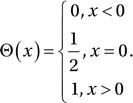
Another useful decorator in the Numba library is numba.vectorize. It generates and JIT compiles a vectorized function from a kernel function written for scalar input and output, much like the NumPy vectorize function. Consider the Heaviside step function
If we wanted to implement this function for scalar input x, we could use:
In [30]: def py_Heaviside(x):
    ...:     if x == 0.0:
    ...:         return 0.5
    ...:     if x < 0.0:
    ...:         return 0.0
    ...:     else:
    ...:         return 1.0
This function only works for scalar input, and if we want to apply it to an array or list we have to explicitly iterate over the array and apply it to each element:
In [31]: x = np.linspace(-2, 2, 50001)
In [32]: %timeit [py_Heaviside(xx) for xx in x]
100 loops, best of 3: 16.7 ms per loop
This is inconvenient and slow. The NumPy vectorize function solves the inconvenience problem, by automatically wrapping the scalar kernel function into a NumPy-array aware function Numba libraryNumPy-array aware function:
In [33]: np_vec_Heaviside = np.vectorize(py_Heaviside)
In [34]: np_vec_Heaviside(x)
Out[34]: array([ 0.,  0.,  0., ...,  1.,  1.,  1.])
However, the NumPy vectorize function does not solve the performance problem. As we see from benchmarking the np_vec_Heaviside function with %timeit, its performance is comparable to explicitly looping over the array and consecutively calls the py_Heaviside function for each element:
In [35]: %timeit np_vec_Heaviside(x)
100 loops, best of 3: 13.6 ms per loop
Better performance can be achieved by using NumPy array expressions instead of using NumPy vectorize on a scalar kernel written in Python:
In [36]: def np_Heaviside(x):
    ...:     return (x > 0.0) + (x == 0.0)/2.0
In [37]: %timeit np_Heaviside(x)
1000 loops, best of 3: 268 μs per loop
However, even better performance can be achieved using Numba and the vectorize decorator, which takes a list of function signatures for which to generate JIT-compiled code. Here we choose to generate vectorized functions for two signatures: one that takes arrays of 32-bit floating-point numbers as input and output, defined as numba.float32(numba.float32), and one that takes arrays of 64-bit floating-point numbers as input and output, defined as numba.float64(numba.float64):
In [38]: @numba.vectorize([numba.float32(numba.float32),
    ...:                   numba.float64(numba.float64)])
    ...: def jit_Heaviside(x):
    ...:     if x == 0.0:
    ...:         return 0.5
    ...:     if x < 0:
    ...:         return 0.0
    ...:     else:
    ...:         return 1.0
Benchmarking the resulting jit_Heaviside function shows the best performance of the methods we have looked at:
In [39]: %timeit jit_Heaviside(x)
10000 loops, best of 3: 58.5 μs per loop
and the jit_Heaviside function can be used as any NumPy universal function Numba libraryNumPy universal function, including support for broadcasting and other NumPy features. To demonstrate that the function indeed implements the desired function we can test it on a simple list on input values:
In [40]: jit_Heaviside([-1, -0.5, 0.0, 0.5, 1.0])
Out[40]: array([ 0. ,  0. ,  0.5,  1. ,  1. ])
In this section we have explored speeding up Python code using JIT compilation with the Numba library. We looked at four examples: two simple examples for demonstrating the basic usage of Numba, the summation and accumulative summation of an array. For a more realistic use-case of Numba that is not so easily defined in terms of vector expressions, we looked at the computation of the Julia set. Finally, we explored the vectorization of scalar kernel with the implementation of the Heaviside step function. These examples demonstrate common use patterns for Numba, but there is also much more to explore in the Numba library, such as code generation for GPUs. For more information about this and other topics, see the official Numba documentation at http://numba.pydata.org/doc.html.
Cython
Like Numba, Cython is a solution for speeding up Python code, although Cython takes a completely different approach to this problem. Whereas Numba is a Python library that converts pure Python code to LLVM code that is JIT compiled into machine code, Cython is a programming language that is a superset of the Python programming language: Cython extends Python with C-like properties. Most notably, Cython allow us to use explicit and static type declarations. The purpose of the extensions to Python introduced in Cython is to make it possible to translate the code into efficient C or C++ code, which can be compiled into a Python extension module that can be imported and used from regular Python code.
There are two main usages of Cython: speeding up Python code and generating wrappers for interfacing with compiled libraries. When using Cython, we need to modify the targeted Python code, so compared to using Numba there is a little bit more work involved, and we need to learn the syntax and behavior of Cython in order to use it to speed up Python code. However, as we will see in this section, Cython provides more fine-grained control of how the Python code is processed, and Cython also has features that are out-of-scope for Numba, such as generating interfaces between Python and external libraries, and speeding up Python code that does not use NumPy arrays.
While Numba uses transparent just-in-time compilation, Cython is mainly designed for using traditional ahead-of-time compilation. There are several ways to compile Cython code into a Python extension module, each with different use-cases. We begin with reviewing options for compiling Cython code, and then proceed to introduce features of Cython that are useful for speeding up computations written in Python. Throughout this section we will work with mostly the same examples that we looked at in the previous section using Numba, so that we can easily compare both the methods and the results. We begin with looking at how to speed up the py_sum and py_cumsum functions defined in the previous section.
To use Cython code from Python it has to pass through the Cython compilation pipeline: First the Cython code must be translated into C or C++ code, after which it has to be compiled into machine code using a C or C++ compiler. The translation from Cython code to C or C++ can be done using the cython command-line tool. It takes a file with Cython code, which we typically store in files using the pyx file extension, and produces a C or C++ file. For example, consider the file cy_sum.pyx, with the content shown in Listing 19-1. To generate a C file from this Cython file, we can run the command cython cy_sum.pyx. The result is the file cy_sum.c, which we can compile using a standard C compiler into a Python extension module. This compilation step is platform dependent, and requires using the right compiler flags and options as to produce a proper Python extension.
To avoid the complications related to platform specific compilation options for C and C++ code we can use the distutils and Cython libraries to automate the translation of Cython code into a useful Python extension module. This requires creating a setup.py script that calls the setup function from distutils.core (which knows how to compile C code into a Python extension) and the cythonize function from Cython.Build (which knows how to translate Cython code into C code), as shown in Listing 19-2. When the setup.py file is prepared, we can compile the Cython module using the command python setup.py build_ext --inplace, which instructs distutils to build the extension module and place it in the same directory as the source code.
Once the Cython code has been compiled into a Python extension module, whether by hand or using distutils library, we can import it and use it as a regular module in Python:
In [41]: from cy_sum import cy_sum
In [42]: cy_sum(data)
Out[42]: -189.70046227549025
In [43]: %timeit cy_sum(data)
100 loops, best of 3: 5.56 ms per loop
In [44]: %timeit py_sum(data)
100 loops, best of 3: 8.08 ms per loop
Here we see that for this example, compiling the pure Python code in Listing 19-3 using Cython directly gives a speed-up of about 30%. This is a nice speed-up, but arguably not worth the trouble of going through the Cython compilation pipeline. We will see later how to improve on this speed-up using more features of Cython.
The explicit compilation of Cython code into a Python extension module shown above is useful for distributing prebuilt modules written in Cython, as the end result does not require Cython to be installed to use the extension module. An alternative way to implicitly invoke the Cython compilation pipeline automatically during the import of a module is provided by the pyximport library, which is distributed with Cython. To seamlessly import a Cython file directly from Python, we can first invoke the install function from the pyximport library:
In [45]: pyximport.install(setup_args=dict(include_dirs=np.get_include()))
This will modify the behavior or the Python import statement, and add support for Cython pyx files. When a Cython module is imported, it will first be compiled in C or C++, and then to machine code in the format of a Python extension module that the Python interpreter can import. These implicit steps sometimes require additional configuration, which we can pass to the pyximport.install function via arguments. For example, to be able to import Cython code that uses NumPy related features we need the resulting C code to be compiled against the NumPy C header files. We can configure this by setting the include_dirs to the value given by np.get_include() in the setup_args argument to the install function, as shown above. Several other options are also available, and we can also give custom compilation and linking arguments. See the docstring for pyximport.install for details. Once pyximport.install has been called, we can use a standard Python import statement to import a function from a Cython module:
In [46]: from cy_cumsum import cy_cumsum
In [47]: %timeit cy_cumsum(data)
100 loops, best of 3: 5.91 ms per loop
In [48]: %timeit py_cumsum(data)
100 loops, best of 3: 13.8 ms per loop
In this example, too, we see a welcome but not very impressive speed-up of a factor of two for the Python code that has been passed through the Cython compilation pipeline.
Before we get into the detailed uses of Cython that allow us to improve upon this speed-up factor, we quickly introduce yet another way of compiling and import Cython code. When using IPython, and especially the IPython notebook, we can use the convenient %%cython command, which automatically compiles and loads Cython code in a code cell as Python extension and makes it available in the IPython session. To be able to use this command, we first have to activate it using the %load_ext cython command:
In [49]: %load_ext cython
With the %%cython command activated, we can write and load Cython code interactively in an IPython session:
In [50]: %%cython
    ...: def cy_sum(data):
    ...:     s = 0.0
    ...:     for d in data:
    ...:         s += d
    ...:     return s
In [51]: %timeit cy_sum(data)
100 loops, best of 3: 5.21 ms per loop
In [52]: %timeit py_sum(data)
100 loops, best of 3: 8.6 ms per loop
As before, see a direct speed-up by simply adding the %%cython at the first line of the IPython code cell. This is reminiscent of adding the @numba.jit decorator to a function, but the underlying mechanics of these two methods are rather different. In the rest of this section we will use this method for compiling and loading Cython code. When using the %%cython IPython command, it is also useful to add the -a argument. This results in Cython annotation output to be displayed as output of the code cell, as shown in Figure 19-2. The annotation shows each code line in a shade of yellow, where bright yellow indicates that the line of code is translated to C code with strong dependencies on the Python C/API, and a where a white line of code is directly translated into pure C code. When working on optimizing Cython code, we generally need to strive for Cython code that gets translated into as pure C code as possible, so it is extremely useful to inspect the annotation output and look for yellow lines, which typically represent the bottlenecks in the code. As an added bonus, clicking on a line of code in the annotation output toggles between the Cython code that we provided and the C code that it is being translated into.
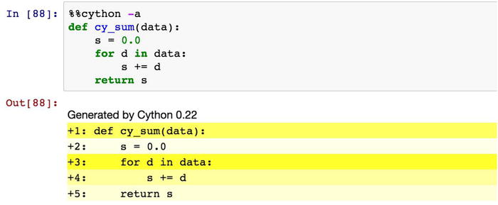
Figure 19-2. Annotation generated by Cython using the %%cython IPython command with the -a argument
In the rest of the section we explore ways of speeding Cython code using language features that is introduced by Cython that are particularly useful for computational problems. We first revisit implementation of the cy_sum given above. In our first attempt to speed up this function we simply used the pure Python passed it through the Cython compilation pipeline, and as a result we saw a speed-up of about 30%. The key step to see much larger speedups is to add type declarations for all the variables and arguments of the function. By explicitly declaring the types of variables the Cython compiler will be able to generate more efficient C code. To specify a type of a variable we need to use the Cython keyword cdef, which we can use with any standard C type. For example, to declare the variable n of integer type, we can use cdef int n. We can also use type definitions from the NumPy library: For example, cdef numpy.float64_t s declares the variable s to be a 64-bit floating-point number. NumPy arrays can be declared using the type specification on the format numpy.ndarray[numpy.float64_t, ndim=1] data, which declare data to be an array with 64-bit floating-point number elements, with one dimension (a vector) and of unspecified length. Adding type declarations of this style to the previous cy_sum function results in the following code:
In [53]: %%cython
    ...: cimport numpy
    ...: cimport cython
    ...:
    ...: @cython.boundscheck(False)
    ...: @cython.wraparound(False)
    ...: def cy_sum(numpy.ndarray[numpy.float64_t, ndim=1] data):
    ...:     cdef numpy.float64_t s = 0.0
    ...:     cdef int n, N = len(data)
    ...:     for n in range(N):
    ...:         s += data[n]
    ...:     return s
In this implementation of the cy_sum function, we have also applied the two decorators @cython.boundscheck(False) and @cython.wraparound(False), which disables time-consuming bound checks on the indexing of NumPy arrays. This result in less safe code, but if we are confident that the NumPy arrays in this function will not be indexed outside of their valid ranges, we can obtain additional speed-up by disable such checks. Now that we have explicitly declared the type of all variables and arguments of the function, Cython is able to generate efficient C code that when compiled into a Python module provides performance that is comparable to the JIT-compiled code using Numba, and not far from the built-in sum function from NumPy (which also is implemented in C):
In [54]: %timeit cy_sum(data)
10000 loops, best of 3: 49.2 μs per loop
In [55]: %timeit jit_sum(data)
10000 loops, best of 3: 47.6 μs per loop
In [56]: %timeit np.sum(data)
10000 loops, best of 3: 29.7 μs per loop
Next let’s turn our attention to the cy_cumsum function. Like the cy_sum function, this function too will befit from explicit type declarations. To simplify the declarations of NumPy array types, here we use the ctypedef keyword to create an alias for numpy.float64_t to the shorter FTYPE_t. Note also that in Cython code, there are two different import statements: cimport and import. The import statement can be used to import any Python module, but it will result in C code that calls back into the Python interpreter, and can therefore be slow. The cimport statement work like a regular import, but is used for importing other Cython modules. Here cimport numpy imports a Cython module named numpy that provides Cython extensions to NumPy; mostly type and function declarations. In particular, the C-like types such numpy.float64_t are declared in this Cython module. However, the function call numpy.zeros in the function defined below results in a call to the function zeros in the NumPy module, and for it we need to include the Python module numpy using import numpy.
Adding these type declarations to the previously defined cy_cumsum function results in the implementation given below:
In [57]: %%cython
    ...: cimport numpy
    ...: import numpy
    ...: cimport cython
    ...:
    ...: ctypedef numpy.float64_t FTYPE_t
    ...:
    ...: @cython.boundscheck(False)
    ...: @cython.wraparound(False)
    ...: def cy_cumsum(numpy.ndarray[FTYPE_t, ndim=1] data):
    ...:     cdef int N = data.size
    ...:     cdef numpy.ndarray[FTYPE_t, ndim=1] out = numpy.zeros(N, dtype=data.dtype)
    ...:     cdef numpy.float64_t s = 0.0
    ...:     for n in range(N):
    ...:         s += data[n]
    ...:         out[n] = s
    ...:     return out
Like for cy_sum, we see a significant speed-up after having declared the types of all variables in the function, and the performance of cy_cumsum is now comparable to the JIT-compiled Numba function jit_cumsum and the faster than the built-in cumsum function in NumPy (which on the other hand is more versatile):
In [58]: %timeit cy_cumsum(data)
10000 loops, best of 3: 69.7 μs per loop
In [59]: %timeit jit_cumsum(data)
10000 loops, best of 3: 70 μs per loop
In [60]: %timeit np.cumsum(data)
10000 loops, best of 3: 148 μs per loop
When adding explicit type declarations we gain performance when compiling the function with Cython, but we lose generality as the function is now unable to take any other type of arguments. For example, original py_sum function, as well as the NumPy sum function, accept a much wider variety of input types. We can sum Python lists and NumPy arrays of both floating-point numbers and integers:
In [61]: py_sum([1.0, 2.0, 3.0, 4.0, 5.0])
Out[61]: 15.0
In [62]: py_sum([1, 2, 3, 4, 5])
Out[62]: 15
The Cython compiled version with explicit type declaration, on the other hand, only works for exactly the type we declared it:
In [63]: cy_sum(np.array([1.0, 2.0, 3.0, 4.0, 5.0]))
Out[63]: 15.0
In [64]: cy_sum(np.array([1, 2, 3, 4, 5]))
---------------------------------------------------------------------------
ValueError: Buffer dtype mismatch, expected 'float64_t' but got 'long'
Often it is desirable support more than one type of input, such as providing the ability to sum arrays of both floating-point numbers and integers with the same function. Cython provides a solution to this problem through its ctypedef fused keyword, with which we can define new types that are one out of several provided types. For example, consider the modification to the py_sum function given in py_fused_sum here:
In [65]: %%cython
    ...: cimport numpy
    ...: cimport cython
    ...:
    ...: ctypedef fused I_OR_F_t:
    ...:     numpy.int64_t
    ...:     numpy.float64_t
    ...:
    ...: @cython.boundscheck(False)
    ...: @cython.wraparound(False)
    ...: def cy_fused_sum(numpy.ndarray[I_OR_F_t, ndim=1] data):
    ...:     cdef I_OR_F_t s = 0
    ...:     cdef int n, N = len(data)
    ...:     for n in range(N):
    ...:         s += data[n]
    ...:     return s
Here the function is defined in terms of the type I_OR_F_t, which is defined using ctypedef fused to be either numpy.int64_t or numpy.float64_t. Cython will automatically generate the necessary code for both types of functions, so that we can use the function on both floating-point and integer arrays (at the price of a small decrease in performance):
In [66]: cy_fused_sum(np.array([1.0, 2.0, 3.0, 4.0, 5.0]))
Out[66]: 15.0
In [67]: cy_fused_sum(np.array([1, 2, 3, 4, 5]))
Out[67]: 15
As a final example of how to speed up Python code with Cython, consider again the Python code for generating the Julia set that we looked at in the previous section. To implement a Cython version of this function, we simply take the original Python code and explicitly declare the types of all the variables used in the function, following the procedure we used above. We also add the decorators for disabling index bound checks and wrap around. Here we have both NumPy integer arrays and floating-point arrays as input, so we define the arguments as types numpy.ndarray[numpy.float64_t, ndim=1] and numpy.ndarray[numpy.int64_t, ndim=2], respectively.
The implementation of cy_julia_fractal given below also includes a Cython implementation of the square of the absolute value of a complex number. This function is declared as inline using the inline keyword, which means that the compiler will put the body of the function at every place it is called, rather than creating a function that is called from those locations. This will result in large code, but avoid the overhead of an additional function call. We also define this function using cdef rather than the usual def keyword. In Cython, def defines a function that can be called from Python, while cdef defines a function that can be called from C. Using the cpdef keyword, we can simultaneously define a function that is both callable from C and from Python. As it is written here, using cdef, we cannot call the abs2 function from the IPython session after executing this code cell, but if we change cdef to cpdef we can.
In [68]: %%cython
    ...: cimport numpy
    ...: cimport cython
    ...:
    ...: cdef inline double abs2(double complex z):
    ...:     return z.real * z.real + z.imag * z.imag
    ...:
    ...: @cython.boundscheck(False)
    ...: @cython.wraparound(False)
    ...: def cy_julia_fractal(numpy.ndarray[numpy.float64_t, ndim=1] z_re,
    ...:                      numpy.ndarray[numpy.float64_t, ndim=1] z_im,
    ...:                      numpy.ndarray[numpy.int64_t, ndim=2] j):
    ...:     cdef int m, n, t, M = z_re.size, N = z_im.size
    ...:     cdef double complex z
    ...:     for m in range(M):
    ...:         for n in range(N):
    ...:             z = z_re[m] + 1.0j * z_im[n]
    ...:             for t in range(256):
    ...:                 z = z ** 2 - 0.05 + 0.68j
    ...:                 if abs2(z) > 4.0:
    ...:                     j[m, n] = t
    ...:                     break
If we call the cy_julia_fractal function with the same arguments as we previously called the Python implementation that was JIT-compiled using Numba, we see that the two implementations have comparable performance.
In [69]: N = 1024
In [70]: j = np.zeros((N, N), dtype=np.int64)
In [71]: z_real = np.linspace(-1.5, 1.5, N)
In [72]: z_imag = np.linspace(-1.5, 1.5, N)
In [73]: %timeit cy_julia_fractal(z_real, z_imag, j)
10 loops, best of 3: 113 ms per loop
In [74]: %timeit jit_julia_fractal(z_real, z_imag, j)
10 loops, best of 3: 141 ms per loop
The slight edge to the cy_julia_fractal implementation is mainly due to the inline definition of the inner-most loops call to the abs2 function, and the fact that abs2 avoids computing the square root. Making a similar change in jit_julia_fractal improves its performance and approximately accounts for the difference shown here.
So far we have explored Cython as a method to speed up Python code by compiling it to machine codes that are made available as Python extension modules. There is another important use-case of Cython, which is at least as important to its widespread use in the Python scientific computing community: Cython can also be used to easily create wrappers to compiled C and C++ libraries. We will not explore this in depth here, but will give a simple example that illustrates that using Cython we can call out to arbitrary C libraries in just a few lines of code. As an example, consider the math library from the C standard library. It provides mathematical functions, similar to those defined in the Python standard library with the same name: math. To use these functions in a C program, we would include the math.h header file to obtain their declarations, and compile and link the program against the libm library. From Cython we can obtain function declarations using the cdef extern from keywords, after which we need to give the name of the C header file and list the declarations of the function we want to use in the following code block. For example, to make the acos function from libm available in Cython, we can use the following code:
In [75]: %%cython
    ...: cdef extern from "math.h":
    ...:     double acos(double)
    ...:
    ...: def cy_acos1(double x):
    ...:     return acos(x)
Here we also defined the Python function cy_acos1, which we can call from Python:
In [76]: %timeit cy_acos1(0.5)
10000000 loops, best of 3: 83.2 ns per loop
Using this method we can wrap arbitrary C functions into functions that are callable from regular Python code. This is a very useful feature for scientific computing applications, since it makes existing code written in C and C++ easily available from Python. For the standard libraries, Cython already provides type declarations via the libc module, so we do not need to explicitly define the functions using cdef extern from. For the acos example, we could therefore instead directly import the function from libc.math using the cimport statement:
In [77]: %%cython
    ...: from libc.math cimport acos
    ...:
    ...: def cy_acos2(double x):
    ...:     return acos(x)
In [78]: %timeit cy_acos2(0.5)
10000000 loops, best of 3: 85.6 ns per loop
The resulting function cy_acos2 is identical to cy_acos1 that was explicitly imported from math.h earlier. It is instructive to compare the performance of these C math library functions to the corresponding functions defined in NumPy and the Python standard math library:
In [79]: from numpy import arccos
In [80]: %timeit arccos(0.5)
1000000 loops, best of 3: 1.07 μs per loop
In [81]: from math import acos
In [82]: %timeit acos(0.5)
10000000 loops, best of 3: 95.9 ns per loop
The NumPy version is about 10 times slower than the Python math function and Cython wrappers to the C standard library function, because of the overhead related to NumPy array data structures.
Summary
In this chapter we have explored methods for speeding up Python code using Numba, which produces optimized machine code using just-in-time compilation; and Cython, which produces C code that can be compiled into machine code using ahead-of-time compilation. Numba works with pure Python code, but heavily relies of type interference using NumPy arrays, while Cython works with an extension to the Python language that allows explicit type declarations. The advantages of these methods are that we can achieve performance that is comparable to compiled machine code, while staying in a Python or Python-like programming environment. The key to the speeding up of Python code is the use of typed variables, either by using type interference from NumPy arrays, as in Numba, or by explicitly declaring the types of variables, as in Cython. Explicitly typed code can be translated into much more efficient code than the dynamically typed code in pure Python, and can avoid much of the overhead involved in type look-ups in Python. Both Numba and Cython are convenient ways to obtain impressive speedups of Python code, and they often produce code with similar performance. Cython also provides an easy-to-use method for creating interfaces to external libraries so that they can be accessed from Python. In both Numba and Cython, the common theme is use type information (from NumPy arrays or from explicit declarations) to generate more efficient typed machine code. Within the Python community, there has also recently been movement toward adding support for optional type hints to the Python language itself. For details about the current status of type hints see PEP 484 (https://www.python.org/dev/peps/pep-0484), which is scheduled to be included in a future release of Python. While type hints in Python is not likely to be widely available in the near future, it is certainly an interesting development to follow.
Further Reading
Thorough guides to using Cython are given in books by Smith and Herron. For more information about Numba, see its official documentation at http://numba.pydata.org/doc.html. For a detailed discussion of high-performance computing with Python, see also the book by Gorelick.
References
Gorelick, I. O. (2014). High Performance Python: Practical Performant Programming for Humans. Sebastopol: O’Reilly.
Herron, P. (2013). Learning Cython Programming. Mumbai: Packt.
Smith, K. (2015). Cython: A Guide for Python Programmers. Sebastopol: O’Reilly.
________________
2http://docs.scipy.org/doc/numpy-dev/f2py/index.html.
3The producers of the Anaconda Python environment, see Chapter 1 and Appendix 1.