![]()
Bayesian Statistics
In this chapter we explore an alternative interpretation of statistics – Bayesian statistics – and the methods associated with this interpretation. Bayesian statistics, in contrast to the frequentist’s statistics that we used in Chapter 13 and Chapter 14, treat probability as a degree of belief rather than as a measure of proportions of observed outcomes. This different point of view gives rise to distinct statistical methods that can be used in problem solving. While it is generally true that statistical problems can in principle be solved using either frequentist or Bayesian statistics, there are practical differences that make these two approaches to statistics suitable for different types of problems.
Bayesian statistics is based on Bayes theorem, which relates conditional and unconditional probabilities. Bayes theorem is a fundamental result in probability theory, and it applies to both the frequentist’s and the Bayesian interpretation of statistics. In the context of Bayesian inference, unconditional probabilities are used to describe the prior knowledge of a system, and Bayes theorem provides a rule for updating this knowledge after making new observations. The updated knowledge is described by a conditional probability, which is conditioned on the observed data. The initial knowledge of a system is described by the prior probability distribution, and the updated knowledge, conditioned on the observed data, is the posterior probability distribution. In problem solving with Bayesian statistics, the posterior probability distribution is the unknown quantity that we seek, and from it we can compute expectation values and other statistical quantities for random variables of interest. Although Bayes theorem describes how to compute the posterior distribution from the prior distribution, for most realistic problems the calculations involve evaluating high-dimensional integrals that can be prohibitively difficult to compute, both analytically and numerically. This has until recently hindered Bayesian statistics from being widely used in practice. However, with the advent of computational statistics, and the development of efficient simulation methods that allows us to sample directly from the posterior distributions (rather than directly compute it), Bayesian methods are becoming increasingly popular. The methods that enable us to sample from the posterior distribution are, first and foremost, the so-called Markov Chain Monte Carlo (MCMC) methods. Several alternative implementations of MCMC methods are available. For instance, traditional MCMC methods include Gibbs sampling and the Metropolis-Hastings algorithm, and more recent methods include Hamiltonian and No-U-Turn algorithms. In this chapter we explore how to use several of these methods.
Statistical problem solving with Bayesian inference methods is sometimes known as probabilistic programming. The key steps in probabilistic programming are the following: (1) Create a statistical model. (2) Sample from the posterior distribution for the quantity of interest using an MCMC method. (3) Use the obtained posterior distribution to compute properties of interest for the problem at hand, and make inference decisions based on the obtained results. In this chapter we explore how to carry out these steps from within the Python environment, with the help of the PyMC library.
![]() pymc The PyMC library provides a framework for doing probabilistic programming – that is, solving statistical problems using simulation with Bayesian methods. At the time of writing, the latest official release is version 2.3. However, the development version for PyMC 3.0 has been in pre-release status quite some time now, and is hopefully released in the near future. Regardless of its release status, the current alpha version of PyMC 3.0 is already very useful and readily available, and it has several advantages over version 2.3 in both the available solvers and the programming style and API. Therefore, in spite of it not being officially released yet, in this chapter we focus on the upcoming version 3.0 of PyMC. However, this also means that some of the code examples shown here might need minor adjustments to work with version 3 of PyMC when it is finally released. For more information about the project, see the web pages at https://pymc-devs.github.io/pymc and https://pymc-devs.github.io/pymc3.
pymc The PyMC library provides a framework for doing probabilistic programming – that is, solving statistical problems using simulation with Bayesian methods. At the time of writing, the latest official release is version 2.3. However, the development version for PyMC 3.0 has been in pre-release status quite some time now, and is hopefully released in the near future. Regardless of its release status, the current alpha version of PyMC 3.0 is already very useful and readily available, and it has several advantages over version 2.3 in both the available solvers and the programming style and API. Therefore, in spite of it not being officially released yet, in this chapter we focus on the upcoming version 3.0 of PyMC. However, this also means that some of the code examples shown here might need minor adjustments to work with version 3 of PyMC when it is finally released. For more information about the project, see the web pages at https://pymc-devs.github.io/pymc and https://pymc-devs.github.io/pymc3.
Importing Modules
In this chapter we mainly work with the pymc3 library, which we import in the following manner:
In [1]: import pymc3 as mc
We also require NumPy, Pandas, and Matplotlib for basic numerics, data analytics, and plotting, respectively. These libraries are imported following the usual convention:
In [2]: import numpy as np
In [3]: import pandas as pd
In [4]: import matplotlib.pyplot as plt
For comparison to non-Bayesian statistics we also use the stats module from SciPy, the statsmodels library, and the Seaborn library for visualization:
In [5]: from scipy import stats
In [6]: import statsmodels.api as sm
In [7]: import statsmodels.formula.api as smf
In [8]: import seaborn as sns
Introduction to Bayesian Statistics
The foundation of Bayesian statistics is the Bayes theorem, which gives a relation between unconditioned and conditional probabilities of two events A and B:
![]()
where P(A) and P(B) are the unconditional probabilities of event A and B, and where ![]() is the conditional probability of event A given that event B is true, and
is the conditional probability of event A given that event B is true, and ![]() is the conditional probability of B given that A is true. Both sides of the equation above are equal to the probability that both A and B are true:
is the conditional probability of B given that A is true. Both sides of the equation above are equal to the probability that both A and B are true: ![]() . In other words, Bayes rule states that the probability that both A and B is equal to the probability of A times the probability of B given that A is true:
. In other words, Bayes rule states that the probability that both A and B is equal to the probability of A times the probability of B given that A is true: ![]() , or, equivalently, the probability of B times the probability of A given B:
, or, equivalently, the probability of B times the probability of A given B: ![]() .
.
In the context of Bayesian inference, Bayes rule is typically employed for the situation when we have prior belief about the probability of an event A, represented by the unconditional probability P(A), and wish to update this belief after having observed an event B. In this language the updated belief is represented by the conditional probability of A given the observation B: ![]() , which we can compute using Bayes rule:
, which we can compute using Bayes rule:
![]()
Each factor in this expression has a distinct interpretation and a name: P(A) is the prior probability of event A, and ![]() is the posterior probability of A given the observation B.
is the posterior probability of A given the observation B. ![]() is the likelihood of observing B given that A is true, and the probability of observing B regardless of A, P(B), is known as model evidence, and can be considered as a normalization constant (with respect to A).
is the likelihood of observing B given that A is true, and the probability of observing B regardless of A, P(B), is known as model evidence, and can be considered as a normalization constant (with respect to A).
In statistical modeling we are typically interested in a set of random variables X that are characterized by probability distributions with certain parameters θ. After collecting data for the process that we are interested in modeling, we wish to infer the values of the model parameters from the data. In the frequentist’s statistical approach, we can maximize the likelihood function given the observed data, and obtain estimators for the model parameters. The Bayesian approach is to consider the unknown model parameters θ as random variables in their own right, and use Bayes rule to derive probability distributions for the model parameters θ. If we denote the observed data as x, we can express the probability distribution for θ given the observed data x using Bayes rule as

The second equality in this equation follows from the law of total probability, ![]() . Once we have computed the posterior probability distribution
. Once we have computed the posterior probability distribution ![]() for the model parameters, we can for compute expectation values of the model parameters and obtain a result that is similar to the estimators that we can compute in a frequentist’s approach. In addition, when we have an estimate of the full probability distribution for
for the model parameters, we can for compute expectation values of the model parameters and obtain a result that is similar to the estimators that we can compute in a frequentist’s approach. In addition, when we have an estimate of the full probability distribution for ![]() we can also compute other quantities, such as credibility intervals, and marginal distributions for certain model parameters in the case when θ is multivariate. For example, if we have two model parameters,
we can also compute other quantities, such as credibility intervals, and marginal distributions for certain model parameters in the case when θ is multivariate. For example, if we have two model parameters, ![]() , but are interested only in θ1, we can obtain the marginal posterior probability distribution
, but are interested only in θ1, we can obtain the marginal posterior probability distribution ![]() by integrating the joint probability distribution
by integrating the joint probability distribution ![]() using the expression obtained from Bayes theorem:
using the expression obtained from Bayes theorem:

Here note that the final expression contains integrals over the known likelihood function ![]() and the prior distribution p(θ1, θ2), so we do not need to know the joint probabilty distribution
and the prior distribution p(θ1, θ2), so we do not need to know the joint probabilty distribution ![]() to compute the marginal probability distribution
to compute the marginal probability distribution ![]() . This approach provides a powerful and generic methodology for computing probability distributions for model parameters and successively updating the distributions once new data becomes available. However, directly computing
. This approach provides a powerful and generic methodology for computing probability distributions for model parameters and successively updating the distributions once new data becomes available. However, directly computing ![]() , or the marginal distributions thereof, requires that we can write down the likelihood function
, or the marginal distributions thereof, requires that we can write down the likelihood function ![]() and the prior distribution p(θ), and that we can evaluate the resulting integrals. For many simple but important problems, it is possible to analytically compute these integrals, and find exact closed-form expressions for the posterior distribution. Textbooks such as Gelman’s (Gelman, 2013) provides numerous examples of problems that are exactly solvable in this way. However, for more complicated models, with prior distributions and likelihood functions for which the resulting integrals are not easily evaluated, or for multivariate statistical models, for which the resulting integrals can be high dimensional, both exact and numerical evaluation may be unfeasible.
and the prior distribution p(θ), and that we can evaluate the resulting integrals. For many simple but important problems, it is possible to analytically compute these integrals, and find exact closed-form expressions for the posterior distribution. Textbooks such as Gelman’s (Gelman, 2013) provides numerous examples of problems that are exactly solvable in this way. However, for more complicated models, with prior distributions and likelihood functions for which the resulting integrals are not easily evaluated, or for multivariate statistical models, for which the resulting integrals can be high dimensional, both exact and numerical evaluation may be unfeasible.
It is primarily for models that cannot be solved with exact methods that we can benefit from using simulation methods, such as Markov Chain Monte Carlo, which allows us to sample the posterior probability distribution for the model parameters, and thereby construct an approximation of the joint or marginal posterior distributions, or directly evaluating integrals, such as expectation values. Another important advantage of simulation-based methods is that the modeling process can be automated. Here we exclusively focus on Bayesian statistical modeling using Monte Carlo simulation methods. For a thorough review of the theory, and many examples of analytically solvable problems, see the references given at the end of this chapter. In the remaining part of this chapter, we explore the definition of statistical models and sampling of their posterior distribution with the PyMC library as a probabilistic programming framework.
Before we proceed with computational Bayesian statistics, it is worth taking a moment to summarize the key differences between the Bayesian approach and the classical frequentist’s approach that we used in earlier chapters. In both approaches to statistical model, we formulate the models in terms of random variables. A key step in the definition of a statistical model is to make assumptions about the probability distributions for the random variables that are defined in the model. In parametric methods, each probability distribution is characterized by a small number of parameters. In the frequentist’s approach, those model parameters have some specific true values, and observed data is interpreted as random samples from the true distributions. In other words, the model parameters are assumed to be fixed, and the data is assumed to be stochastic. The Bayesian approach takes the opposite point of view: The data is interpreted as fix, and the model parameters are described as random variables. Starting from a prior distribution for the model parameters, we can then update the distribution to account for observed data, and in the end obtain a probability distribution for the relevant model parameters, conditioned on the observed data.
Model Definition
A statistical model is defined in terms of a set of random variables. The random variables in a given model can be independent or, more interestingly, dependent on each other. The PyMC library provides classes for representing random variables for a large number of probability distributions: For example, an instance of mc.Normal can be used to represent a normal-distributed random variable. Other examples are mc.Bernoulli for representing discrete Bernoulli distributed random variables, mc.Uniform for uniformly distributed random variables, mc.Gamma for Gamma-distributed random variables, and so on. For a complete list of available distributions, see dir(mc.distributions) and the docstrings for each available distribution for information on how to use them. It is also possible to define custom distributions using the mc.DensityDist class, which takes a function that specifies the logarithm of the random variable’s probability density function.
In Chapter 13 we saw that the SciPy stats module also contains classes for representing random variables. Like the random variable classes in SciPy stats, we can use the PyMC distributions to represent random variables with fixed parameters. However, the essential feature of the PyMC random variables is that the distribution parameters, such as the mean μ and variance σ2 for a random variable following the normal distribution ![]() , can themselves be random variables. This allows us to chain random variables in a model, and to formulate models with hierarchical structure in the dependencies between random variables that occur in the model.
, can themselves be random variables. This allows us to chain random variables in a model, and to formulate models with hierarchical structure in the dependencies between random variables that occur in the model.
Let’s start with the simplest possible example. In PyMC, models are represented by an instance of the class mc.Model, and random variables are added to a model using the Python context syntax: Random variable instances that are created within the body of a model context are automatically added to the model. Say that we are interested in a model consisting of a single random variable that follows the normal distribution with the fixed parameters ![]() and
and ![]() . We first define the fixed model parameters, and then create an instance of mc.Model to represent our model.
. We first define the fixed model parameters, and then create an instance of mc.Model to represent our model.
In [9]: mu = 4.0
In [10]: sigma = 2.0
In [11]: model = mc.Model()
Next we can attach random variables to the model by creating them within the model context. Here, we create a random variable X within the model context, which is activated using a with model statement:
In [12]: with model:
    ...:     mc.Normal('X', mu, 1/sigma**2)
All random variable classes in PyMC takes as first argument the name of the variable. In the case of mc.Normal, the second argument is the mean of the normal distribution, and the third argument is the precision ![]() , where σ2 is the variance. Alternatively, we can use the sd keyword argument to specify the standard deviation rather than precision: mc.Normal('X', mu, sd=sigma).
, where σ2 is the variance. Alternatively, we can use the sd keyword argument to specify the standard deviation rather than precision: mc.Normal('X', mu, sd=sigma).
We can inspect which random variables exist in a model using the vars attribute. Here we have only one random variable in the model:
In [13]: model.vars
Out[13]: [X]
To sample from the random variables in the model, we use the mc.sample function, which implements the MCMC algorithm. The mc.sample function accepts many arguments, but at a minimum we need to provide the number of samples as first argument, and as second argument a step-class instance, which implements an MCMC step. Optionally we can also provide a starting point as a dictionary with parameter values from which the sampling is started, using the start keyword argument. For the step method, here we use an instance of the Metropolis class, which implements the Metropolis-Hasting step method for the MCMC sampler.1 Note that we execute all model-related code within the model context:
In [14]: start = dict(X=2)
In [15]: with model:
    ...:     step = mc.Metropolis()
    ...:     trace = mc.sample(10000, start=start, step=step)
[-----------------100%-----------------] 10000 of 10000 complete in 1.6 sec
With these steps we have sampled 10,000 values from the random variable defined within the model, which in this simple case is only a normal-distributed random variable. To access the samples we can use the get_values method of the trace object returned by the mc.sample function:
In [16]: X = trace.get_values("X")
The probability density function (PDF) for a normal distributed is, of course, known analytically. Using SciPy stats module, we can access the PDF using the pdf method of the norm class instance for comparing to the sampled random variable. The sampled values and the true PDF for the present model are shown in Figure 16-1.
In [17]: x = np.linspace(-4, 12, 1000)
In [18]: y = stats.norm(mu, sigma).pdf(x)
In [19]: fig, ax = plt.subplots(figsize=(8, 3)
    ...: ax.plot(x, y, 'r', lw=2)
    ...: sns.distplot(X, ax=ax)
    ...: ax.set_xlim(-4, 12)
    ...: ax.set_xlabel("x")
    ...: ax.set_ylabel("Probability distribution")

Figure 16-1. The probability density function for the normal-distributed random variable (red/thick line), and a histogram from 10,000 MCMC samples of the normal distribution random variable
With the mc.traceplot function we can also visualize the MCMC random walk that generated the samples, as shown in Figure 16-2. The mc.traceplot function automatically plots both the kernel-density estimate and the sampling trace for every random variable in the model.
In [20]: fig, axes = plt.subplots(1, 2, figsize=(8, 2.5), squeeze=False)
    ...: mc.traceplot(trace, ax=axes)
    ...: axes[0,0].plot(x, y, 'r', lw=0.5)

Figure 16-2. Left panel: The kernel-density estimate (blue/thick line) of the sampling trace, and the normal probability distribution (red/thin line). Right panel: the MCMC sampling trace
As a next step in building more complex statistical models, consider a model with a normal-distributed random variable ![]() , but where parameters μ and σ themselves are random variables. In PyMC, we can easily create dependent variables by passing them as argument when creating other random variables. For example, with
, but where parameters μ and σ themselves are random variables. In PyMC, we can easily create dependent variables by passing them as argument when creating other random variables. For example, with ![]() and
and ![]() , we can create the dependent random variable X using the following model specification:
, we can create the dependent random variable X using the following model specification:
In [21]: model = mc.Model()
In [22]: with model:
    ...:     mean = mc.Normal('mean', 3.0)
    ...:     sigma = mc.HalfNormal('sigma', sd=1.0)
    ...:     X = mc.Normal('X', mean, sd=sigma)
Here we have used the mc.HalfNormal to represent the random variable ![]() , and the mean and standard deviation arguments to the mc.Normal class for X are random variable instances rather than fixed model parameters. As before we can inspect which random variables a model contains using the vars attribute.
, and the mean and standard deviation arguments to the mc.Normal class for X are random variable instances rather than fixed model parameters. As before we can inspect which random variables a model contains using the vars attribute.
In [23]: model.vars
Out[23]: [mean, sigma_log, X]
When the complexity of the model increases, it may no longer be straightforward to select a suitable starting point for the sampling process explicitly. The mc.find_MAP function can be used to find the point in the parameter space that corresponds to the maximum of the posterior distribution, which can serve as a good starting point for the sampling process.
In [24]: with model:
    ...:     start = mc.find_MAP()
In [25]: start
Out[25]: {'X': array(3.0), 'mean': array(3.0), 'sigma_log': array(-5.990881458955034)}
As before, once the model is specified, and a starting point is computed, we can sample from the random variables in the model using the mc.sample function, for example, using mc.Metropolis as a MCMC sampling step method:
In [26]: with model:
    ...:     step = mc.Metropolis()
    ...:     trace = mc.sample(100000, start=start, step=step)
[-----------------100%-----------------] 100000 of 100000 complete in 53.4 sec
For example, to obtain the sample trace for the sigma variable we can use get_values('sigma'). The result is a NumPy array that contains the sample values, and from it we can compute further statistics, such as its sample mean and standard deviation:
In [27]: trace.get_values('sigma').mean()
Out[27]: 0.80054476153369014
The same approach can be used to obtain the samples of X and compute statistics from them:
In [28]: X = trace.get_values('X')
In [29]: X.mean()
Out[29]: 2.9993248663922092
In [30]: trace.get_values('X').std()
Out[30]: 1.4065656512676457
The trace plot for the current model, created using the mc.traceplot, is shown in Figure 16-3, where we have used the vars argument to mc.traceplot to explicitly select which random variables to plot.
In [31]: fig, axes = plt.subplots(3, 2, figsize=(8, 6), squeeze=False)
    ...: mc.traceplot(trace, vars=['mean', 'sigma', 'X'], ax=axes)

Figure 16-3. Kernel-density estimates (left) and MCMC random sampling trace (right), for the three random variables: mean, sigma, and X
Sampling Posterior Distributions
So far we have defined models and sampled from models that only contain random variables without any references to observed data. In the context of Bayesian models, these types of random variables represent the prior distributions of the unknown model parameters. In the previous examples we have therefore used the MCMC method to sample from the prior distributions of the model. However, the real application of the MCMC algorithm is to sample from the posterior distribution, which represents the probability distribution for the model variables after having updated the prior distribution to account for the effect of observations.
To condition the model on observed data, all we need to do is to add the data using the observed keyword argument when the corresponding random variable is created within the model. For example, mc.Normal('X', mean, 1/sigma**2, observed=data) indicates that the random variable X has been observed to take the values in the array data. Adding observed random variables to a model automatically results in that subsequent sampling using mc.sample samples the posterior distribution of the model, appropriately conditioned on the observed data according to Bayes rule and the likelihood function implied by the distribution selected for the observed data. For example, consider the model we used above, with a normal-distributed random variable X whose mean and standard deviation are random variables. Here we simulate the observations for X by drawing samples from a normal-distributed random variable with ![]() and
and ![]() using the norm class from the SciPy stats module:
using the norm class from the SciPy stats module:
In [32]: mu = 2.5
In [33]: s = 1.5
In [34]: data = stats.norm(mu, s).rvs(100)
The data is feed into the model by setting the keyword argument observed=data when the observed variable is created and added to the model:
In [35]: with mc.Model() as model:
    ...:     mean = mc.Normal('mean', 4.0, 1.0) # true 2.5
    ...:     sigma = mc.HalfNormal('sigma', 3.0 * np.sqrt(np.pi/2)) # true 1.5
    ...:     X = mc.Normal('X', mean, 1/sigma**2, observed=data)
A consequence of providing observed data for X is that it is no longer considered as a random variable in the model. This can be seen from inspecting the model using the vars attribute, where X is now absent:
In [36]: model.vars
Out[36]: [mean, sigma_log]
Instead, in this case X is a deterministic variable that is used to construct the likelihood function that relates the priors, which are represented by mean and sigma in this case, to the posterior distribution for these random variables. Like before, we can find a suitable starting point for the sampling process using the mc.find_MAP function. After creating an MCMC step instance, we can sample the posterior distribution for the model using mc.sample:
In [37]: with model:
    ...:     start = mc.find_MAP()
    ...:     step = mc.Metropolis()
    ...:     trace = mc.sample(100000, start=start, step=step)
[-----------------100%-----------------] 100000 of 100000 complete in 36.1 sec
The starting point that was calculated using mc.find_MAP maximizes the likelihood of the posterior given the observed data, and it provides an estimate of the unknown parameters of the prior distribution:
In [38]: start
Out[38]: {'mean': array(2.5064940359768246), 'sigma_log': array(0.394681633456101)}
However, to obtain estimates of the distribution of these parameters (which here are random variables in their own right), we need to carry out the MCMC sampling using the mc.sample function, as done above. The result of the posterior distribution sampling is shown in Figure 16-4. Note that the distributions for the mean and sigma variables are closer to the true parameter values, ![]() and
and ![]() , than to the prior guesses of 4.0 and 3.0, respectively, due to the influence of the data and the corresponding likelihood function.
, than to the prior guesses of 4.0 and 3.0, respectively, due to the influence of the data and the corresponding likelihood function.
In [38]: fig, axes = plt.subplots(2, 2, figsize=(8, 4), squeeze=False)
    ...: mc.traceplot(trace, vars=['mean', 'sigma'], ax=axes)

Figure 16-4. The MCMC sampling trace of the posterior distribution for mean and sigma
To calculate statistics and estimate quantities using the samples from the posterior distributions, we can access arrays containing the samples using the get_values method, which takes the name of the random variable as argument. For example, below we compute estimates of the mean of the two random variables in the model, and compare to the corresponding true value from for the distribution that the data points were draw from:
In [39]: mu, trace.get_values('mean').mean()
Out[39]: (2.5, 2.5290001218008435)
In [40]: s, trace.get_values('sigma').mean()
Out[40]: (1.5, 1.5029047840092264)
The PyMC library also provides utilities for analyzing and summarizing the statistics of the marginal posterior distributions obtained from the mc.sample function. For example, the mc.forestplot function visualizes the mean and credibility intervals (that is, and interval within which the true parameter value is likely to be) for each random variable in a model. The result of visualizing the samples for the current example using the mc.forestplot function is shown in Figure 16-5:
In [41]: mc.forestplot(trace, vars=['mean', 'sigma'])
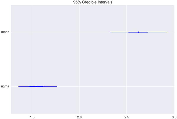
Figure 16-5. A forest plot for the two parameters mean and sigma, which show their credibility intervals
Similar information can also be presented in text form using the mc.summary function, which for includes information such as the mean, standard deviation, and posterior quantiles.
In [42]: mc.summary(trace, vars=['mean', 'sigma'])
mean:

   Mean             SD               MC Error         95% HPD interval
   -------------------------------------------------------------------
   2.472            0.143            0.001            [2.195, 2.757]
   Posterior quantiles:
   2.5            25             50             75             97.5
   |--------------|==============|==============|--------------|
   2.191          2.375          2.470          2.567          2.754

sigma:

   Mean             SD               MC Error         95% HPD interval
   -------------------------------------------------------------------
   1.440            0.097            0.001            [1.256, 1.630]
   Posterior quantiles:
   2.5            25             50             75             97.5
   |--------------|==============|==============|--------------|
   1.265          1.372          1.434          1.501          1.643
Linear Regression
Regression is one of the most basic tools in statistical modeling, and we have already seen examples of linear regression within the classical statistical formalism in Chapters 14 and 15. Linear regression can also be approached with Bayesian methods, and treated as a modeling problem where we assign prior probability distributions to the unknown model parameters (slopes and intercept), and compute the posterior distribution given the available observations. To be able to compare the similarities and differences between Bayesian linear regression and the frequentist’s approach to the same problem, using, for example, the methods from Chapter 14, here we begin with a short analysis of a linear regression problem using the statsmodels library. Next we proceed to analyze the same problem with PyMC.
As example data for performing a linear regression analysis, here we use a dataset that contains the height and weight for 200 men and women, which we can load using the get_rdataset function from the datasets module in the statsmodels library:
In [42]: dataset = sm.datasets.get_rdataset("Davis", "car")
For simplicity, to begin with we work only with the subset of the dataset that corresponds to male subjects, and to avoid having to deal with outliers, we filter out all subjects with weight that exceed 110 kilograms. These operations are readily performed using pandas methods for filtering data frames using Boolean masks:
In [43]: data = dataset.data[dataset.data.sex == 'M']
In [44]: data = data[data.weight < 110]
The resulting pandas data frame object data contains several columns:

Here we focus on a linear regression model for the relationship between the weight and height columns in this dataset. Using the statsmodels library and its model for ordinary least square regression and the Patsy formula language, we create a statistical model for this relationship in a single line of code:
In [46]: model = smf.ols("height ~ weight", data=data)
To actually perform the fitting of the specified model to the observed data, we use the fit method of the model instance:
In [47]: result = model.fit()
Once the model has been fitted and the model result object has been created, we can use the predict method to compute the predictions for new observations, and for plotting the linear relation between the height and weight, as shown in Figure 16-6.
In [48]: x = np.linspace(50, 110, 25)
In [49]: y = result.predict({"weight": x})
In [50]: fig, ax = plt.subplots(1, 1, figsize=(8, 3))
    ...: ax.plot(data.weight, data.height, 'o')
    ...: ax.plot(x, y, color="blue")
    ...: ax.set_xlabel("weight")
    ...: ax.set_ylabel("height")

Figure 16-6. Height versus weight, with a linear model fitted using ordinary least square
The linear relation shown in Figure 16-6 summarizes the main result of performing a linear regression on this dataset. It gives the best fitting line, described by specific values of the model parameters (intercept and slope). Within the frequentist’s approach to statistics, we can also compute numerous statistics, for example, p-values for various hypotheses, such as the hypotheses that a model parameter is zero (no effect).
The end result of a Bayesian regression analysis is the posterior distribution for the marginal distributions for each model parameter. From such marginal distributions we can compute the mean estimates for the model parameters, which roughly correspond to the model parameters obtained from a frequentist’s analysis. We can also compute other quantities, such as the credibility interval, which characterizes the uncertainty in the estimate. To model the height versus weight using a Bayesian model, we can use a relation such as ![]() , where intercept, β, and σ are random variables with unknown distributions and parameters. We also need to give prior distributions to all stochastic variables in the model. Depending on the application, the exact choice of prior can be a sensitive issue, but when there is a lot of data to fit, it is normally sufficient to use reasonable initial guesses. Here we simply start with priors that represent broad distributions for all the model parameters.
, where intercept, β, and σ are random variables with unknown distributions and parameters. We also need to give prior distributions to all stochastic variables in the model. Depending on the application, the exact choice of prior can be a sensitive issue, but when there is a lot of data to fit, it is normally sufficient to use reasonable initial guesses. Here we simply start with priors that represent broad distributions for all the model parameters.
To program the model in PyMC we use the same methodology as earlier in this chapter. First we create random variables for the stochastic components of the model, and assign them to distributions with specific parameters that represent the prior distributions. Next we create a deterministic variable that are functions of the stochastic variables, but with observed data attached to it using the observed keyword argument, as well as in the expression for the expected value of the distribution of the heights (height_mu).
In [51]: with mc.Model() as model:
    ...:     sigma = mc.Uniform('sigma', 0, 10)
    ...:     intercept = mc.Normal('intercept', 125, sd=30)
    ...:     beta = mc.Normal('beta', 0, sd=5)
    ...:     height_mu = intercept + beta * data.weight
    ...:     mc.Normal('height', mu=height_mu, sd=sigma, observed=data.height)
    ...:     predict_height = mc.Normal('predict_height', mu=intercept + beta * x, sd=sigma,
    ...:                                shape=len(x))
If we want to use the model for predicting the heights at specific values of weights, we can also add an additional stochastic variable to the model. In the model specification above, the predict_height variable is an example of this. Here x is the NumPy array with values between 50 and 110 that was created earlier. Because it is an array, we need to set the shape attribute of the mc.Normal class to the corresponding length of the array. If we inspect the vars attribute of the model we now see that it contains the two model parameters (intercept and beta), the distribution of the model errors (sigma), and the predict_height variable for prediction the heights at the specific values weight from the x array:
In [52]: model.vars
Out[52]: [sigma_interval, intercept, beta, predict_height]
Once the model is fully specified, we can turn to the MCMC algorithm to sample the marginal posterior distributions for the model, given the observed data. Like before, we can use mc.find_MAP to find a suitable starting point. Here we use an alternative sampler, mc.NUTS (No U-Turn Sampler), which is a new and powerful sampler that has been added to version 3 of PyMC.
In [53]: with model:
    ...:     start = mc.find_MAP()
    ...:     step = mc.NUTS(state=start)
    ...:     trace = mc.sample(10000, step, start=start)
[-----------------100%-----------------] 10000 of 10000 complete in 43.1 sec
The result of the sampling is stored in a trace object returned by mc.sample. We can visualize the kernel-density estimate of the probability distribution and the MCMC random walk traces that generated the samples using the mc.traceplot function. Here we again use the vars argument to explicitly select which stochastic variables in the model to show in the trace plot. The result is shown in Figure 16-7.
In [54]: fig, axes = plt.subplots(2, 2, figsize=(8, 4), squeeze=False)
    ...: mc.traceplot(trace, vars=['intercept', 'beta'], ax=axes)

Figure 16-7. Distrubution and sampling trace of the linear model intercept and beta coefficient
The values of the intercept and coefficient in the linear model that most closely correspond to the results from the statsmodels analysis above are obtained by computing the mean of the traces for the stochastic variables in the Bayesian model:
In [55]: intercept = trace.get_values("intercept").mean()
In [56]: intercept
Out[56]: 149.97546241676989
In [57]: beta = trace.get_values("beta").mean()
In [58]: beta
Out[58]: 0.37077795098761318
The corresponding result from the statsmodels analysis is obtained by accessing the params attribute in the result class returned by the fit method (see above):
In [59]: result.params
Out[59]: Intercept    152.617348
         weight         0.336477
         dtype: float64
By comparing these values for the intercepts and the coefficients we see that the two approaches gives similar results for the maximum likelihood estimates of the unknown model parameters. In the statsmodels approach, to predict the expected height for a given weight, say 90 kg, we can use the predict method to get a specific height:
In [60]: result.predict({"weight": 90})
Out[60]: array([ 182.90030002])
The corresponding result in the Bayesian model is obtained by computing the mean for the distribution of the stochastic variable predict_height, for the given weight:
In [61]: weight_index = np.where(x == 90)[0][0]
In [62]: trace.get_values("predict_height")[:, weight_index].mean()
Out[62]: 183.33943635274935
Again, the results from the two approaches are comparable. In the Bayesian model, however, we have access to an estimate of the full probability distribution of the height at every modeled weight. For example, we can plot an histogram and the kernel-density estimate of the probability distribution at the weight 90 kg using the distplot function from the Seaborn library, which results in the graph shown in Figure 16-8:
In [63]: fig, ax = plt.subplots(figsize=(8, 3))
    ...: sns.distplot(trace.get_values("predict_height")[:, weight_index], ax=ax)
    ...: ax.set_xlim(150, 210)
    ...: ax.set_xlabel("height")
    ...: ax.set_ylabel("Probability distribution")

Figure 16-8. Probability distribution for prediction of height for weight being 90 kg
Every sample in the MCMC trace represents a possible value of the intercept and coefficients in the linear model that we wish to fit to the observed data. To visualize the uncertainty in the mean intercept and coefficient that we can take as estimates of the final linear model parameters, it is illustrative to plot the lines corresponding to each sample point, along with the data as a scatter plot and the lines that corresponds to the mean intercept and slope. This results in a graph like the one shown in Figure 16-9. The spread of the lines represents the uncertainty in the estimate of the height for a given weight. The spread tends to be larger towards the edges where fewer data points are available, and tighter in the middle cloud of data points.
In [64]: fig, ax = plt.subplots(1, 1, figsize=(8, 3))
    ...: for n in range(500, 2000, 1):
    ...:     intercept = trace.get_values("intercept")[n]
    ...:     beta = trace.get_values("beta")[n]
    ...:     ax.plot(x, intercept + beta * x, color='red', lw=0.25, alpha=0.05)
    ...: intercept = trace.get_values("intercept").mean()
    ...: beta = trace.get_values("beta").mean()
    ...: ax.plot(x, intercept + beta * x, color='k', label="Mean Bayesian prediction")
    ...: ax.plot(data.weight, data.height, 'o')
    ...: ax.plot(x, y, '--', color="blue", label="OLS prediction")
    ...: ax.set_xlabel("weight")
    ...: ax.set_ylabel("height")
    ...: ax.legend(loc=0)

Figure 16-9. Height versus weight, with linear fits using OLS and a Bayesian model
In the linear regression problem we have looked at here, we explicitly defined the statistical model and the stochastic variables included in the model. This illustrates the general steps that are required for analyzing statistical models using the Bayesian approach and the PyMC library. For generalized linear model, however, the PyMC library provides a simplified API that creates the model and the required stochastic variables for us. With the mc.glm.glm function we can define a generalized linear model using Patsy formula (see Chapter 14), and provide the data using a pandas data frame. This automatically takes care of setting up the model. With the model setup using mc.glm.glm, we can proceed to sample from the posterior distribution of the model using the same methods as before.
In [65]: with mc.Model() as model:
    ...:     mc.glm.glm('height ~ weight', data)
    ...:     step = mc.NUTS()
    ...:     trace = mc.sample(2000, step)
[-----------------100%-----------------] 2000 of 2000 complete in 99.1 sec
The result from the sampling of the GLM model, as visualized by the mc.traceplot function, is shown in Figure 16-10. In these trace plots, sd corresponds to the sigma variable in the explicit model definition used above, and it represents the standard error of the residual of the model and the observed data. In the traces, note how the sampling requires a few hundred samples before it reaches a steady level. The initial transient period is does not contribute samples with the correct distribution, so when using the samples to compute estimates we should exclude the samples from the initial period.
In [66]: fig, axes = plt.subplots(3, 2, figsize=(8, 6), squeeze=False)
    ...: mc.traceplot(trace, vars=['Intercept', 'weight', 'sd'], ax=axes)

Figure 16-10. Sample trace plot for a Bayesian GLM model defined using mc.glm module
With the mc.glm.glm we can create and analyze linear models using Bayesian statistics in almost the same way as we define and analyze a model using the frequentist’s approach with statsmodels. For the simple example studied here, the regression analysis with both statistical approaches give similar results and neither methods is much more suitable than the other. However, there are practical differences that depending on the situation can favor one or the other. For example, with the Bayesian approach we have access to estimates of the full marginal posterior distributions, which can be useful for computing statistical quantities other than the mean. However, performing MCMC on simple models like the one considered here is significantly more computationally demanding than carrying out ordinary least square fitting. The real advantages of the Bayesian methods arise when analyzing complicated models in high dimensions (many unknown model parameters). In such cases, defining appropriate frequentist’s models can be difficult, and solving the resulting models challenging. The MCMC algorithm has the very attractive property that is scales well to high-dimensional problems, and can therefore be highly competitive for complex statistical models. While the model we have considered here all are simple, and can easily be solved using a frequentist’s approach, the general methodology used here remains unchanged, and creating more involved models is only a matter of adding more stochastic variables to the model.
As a final example illustrating that the same general procedure can be used also when the complexity of the Bayesian model is increased. We return to the height and weight dataset, but instead of selecting only the male subjects, here we consider an additional level in the model that accounts for the gender of the subject, so that both males and females can be modeled with potentially different slopes and intercepts. In PyMC we can create a multilevel model by using the shape argument to specify the dimension for each stochastic variable that is added to the model, as shown in the following example.
We begin with preparing the dataset. Here we again restricting our analysis to subjects with weight less than 110 kg, to eliminate outliers, and we convert the sex column to a binary variable where 0 represent male and 1 represent female.
In [67]: data = dataset.data.copy()
In [68]: data = data[data.weight < 110]
In [69]: data["sex"] = data["sex"].apply(lambda x: 1 if x == "F" else 0)
Next we define the statistical model, which we here take to be ![]() , where i is an index that takes the value 0 for male subjects and 1 for female subjects. When creating the stochastic variable for the intercept and βi, we indicate this multilevel structure by specifying shape=2 (since in this case we have two levels: male and female). The only other difference compared to the previous model definition is that we also need to use an index mask when defining the expression for height_mu, so that each value in data.weight is associated with the correct level.
, where i is an index that takes the value 0 for male subjects and 1 for female subjects. When creating the stochastic variable for the intercept and βi, we indicate this multilevel structure by specifying shape=2 (since in this case we have two levels: male and female). The only other difference compared to the previous model definition is that we also need to use an index mask when defining the expression for height_mu, so that each value in data.weight is associated with the correct level.
In [70]: with mc.Model() as model:
    ...:     intercept_mu, intercept_sigma = 125, 30
    ...:     beta_mu, beta_sigma = 0, 5
    ...:
    ...:     intercept = mc.Normal('intercept', intercept_mu, sd=intercept_sigma, shape=2)
    ...:     beta = mc.Normal('beta', beta_mu, sd=beta_sigma, shape=2)
    ...:     error = mc.Uniform('error', 0, 10)
    ...:
    ...:     sex_idx = data.sex.values
    ...:     height_mu = intercept[sex_idx] + beta[sex_idx] * data.weight
    ...:
    ...:     mc.Normal('height', mu=height_mu, sd=error, observed=data.height)
Inspecting the model variables using the vars attribute object shows that we again have three stochastic variables in the model: intercept, beta, and error. However, in contrast to the earlier model, here intercept and beta both have two levels.
In [71]: model.vars
Out[71]: [intercept, beta, error_interval]
The way we invoke the MCMC sampling algorithm is identical to the earlier examples in this chapter. Here we use the NUTS sampler, and collect 5000 samples:
In [72]: with model:
    ...:     start = mc.find_MAP()
    ...:     step = mc.NUTS(state=start)
    ...:     trace = mc.sample(5000, step, start=start)
[-----------------100%-----------------] 5000 of 5000 complete in 64.2 sec
We can also, like before, use the mc.traceplot function to visualize the result of the sampling. This allows us to quickly form an idea of the distribution of the model parameters, and to verify that the MCMC sampling has produce sensible results. The trace plot for the current model is shown in Figure 16-11, and unlike earlier examples here we have multiple curves in the panels for the intercept and beta variables, reflecting their multilevel nature: The blue (dark) lines show the results for the male subjects, and the green (light) lines show the result for female subjects.
In [73]: mc.traceplot(trace, figsize=(8, 6))

Figure 16-11. Kernel-density estimate of the probability distribution of the model parameters, and the MCMC sampling traces for each variable in the multilevel model for height versus weight
Using the get_values method of the trace object, we can extract the sampling data for the model variables. Here the sampling data for intercept and beta are two-dimensional arrays with shape (5000, 2): The first dimension represents each sample, and the second dimension represents the level of the variable. Here we are interested in the intercept and the slope for each gender, so we take the mean along the first axis (all samples):
In [74]: intercept_m, intercept_f = trace.get_values('intercept').mean(axis=0)
In [75]: beta_m, beta_f = trace.get_values('beta').mean(axis=0)
By averaging over both dimensions we can also get the intercept and the slope that represent the entire dataset, where male and female subjects are grouped together:
In [76]: intercept = trace.get_values('intercept').mean()
In [77]: beta = trace.get_values('beta').mean()
Finally, we visualize the results by plotting the data as scatter plots, and drawing the lines corresponding to the intercepts and slopes that we obtained for male and female subjects, as well as the result from grouping all subjects together. The result is shown in Figure 16-12.
In [78]: fig, ax = plt.subplots(1, 1, figsize=(8, 3))
    ...: mask_m = data.sex == 0
    ...: mask_f = data.sex == 1
    ...: ax.plot(data.weight[mask_m], data.height[mask_m], 'o', color="steelblue",
    ...:         label="male", alpha=0.5)
    ...: ax.plot(data.weight[mask_f], data.height[mask_f], 'o', color="green",
    ...:         label="female", alpha=0.5)
    ...: x = np.linspace(35, 110, 50)
    ...: ax.plot(x, intercept_m + x * beta_m, color="steelblue", label="model male group")
    ...: ax.plot(x, intercept_f + x * beta_f, color="green", label="model female group")
    ...: ax.plot(x, intercept + x * beta, color="black", label="model both groups")
    ...:
    ...: ax.set_xlabel("weight")
    ...: ax.set_ylabel("height")
    ...: ax.legend(loc=0)

Figure 16-12. The height versus weight for male (dark/blue) and female (light/green) subjects
The regression lines shown in Figure 16-12, and the distribution plots shown in Figure 16-11, indicate that the model is improved by taking account for different intercepts and slopes for male and female subjects. In a Bayesian model with PyMC, changing the underlying model used in the analysis is only a matter of adding stochastic variables to the model, defining how they are related to each other, and assigning a prior distribution for each stochastic variable. The MCMC sampling required to actually solve the model is independent of the model details. This is one of the most attractive aspects of Bayesian statistical modeling. For instance, in the multilevel model considered above, instead of specifying the priors for the intercept and slope variables as independent probability distributions, we could relate the distribution parameters of the priors to another stochastic variable, and thereby obtain a hierarchical Bayesian model, where the model parameters describing the distribution of the intercept and the slope for each level are drawn from a common distribution. Hierarchical models have many uses, and are one of the many applications where Bayesian statistics excels.
Summary
In this chapter we have explored Bayesian statistics using computational methods provided by the PyMC library. The Bayesian approach to statistics is distinct from classical frequentist’s statistics in several fundamental viewpoints. From a practical, computational point of view, Bayesian methods are often very demanding to solve exactly. In fact, computing the posterior distribution for a Bayesian model exactly is often prohibitively expensive. However, what we often can do is to apply powerful and efficient sampling methods that allow us to find an approximate posterior distribution using simulations. The key role of a Bayesian statistics framework is to allow us to define statistical models and then apply sampling methods to find an approximate posterior distribution for the model. In this chapter we have employed the upcoming (but already available) version 3 of the PyMC library as a Bayesian modeling framework in Python. We briefly explored defining statistical models in terms of stochastic variables with given distributions, and the simulation and sampling of the posterior distribution for those models using the MCMC methods implemented in the PyMC library.
Further Reading
For accessible introductions to the theory of Bayesian statistics, see books by Krusche and Downey. A more technical discussion is given in the book by Gelman. A computationally oriented introduction to Bayesian methods with Python is given in “Probabilistic Programming & Bayesian Methods for Hackers,” which is available for free online at http://camdavidsonpilon.github.io/Probabilistic-Programming-and-Bayesian-Methods-for-Hackers. An interesting discussion about the differences between the Bayesian and frequentist’s approaches to statistics, with examples written in Python, is given in the VanderPlas article, which is also available at http://arxiv.org/pdf/1411.5018.pdf.
References
Downey, A. (2013). Think Bayes. Sebastopol: O’Reilly.
Gelman, A. (2013). Bayesian Data Analysis.3rd ed. New York: CRC Press.
Kruschke, J. (2014). Doing Bayesian Data Analysis. Amsterdam: Academic Press.
VanderPlas, J. (2014). “Frequentism and Bayesianism: A Python-Driven Primer.” Proceedings of the 13th Python in Science Conference. Austin: SCIPY.
_________________
1See also the Slice, HamiltonianMC, and NUTS samplers, which can be used more or less interchangeably.