Chapter 10. Underlay and Overlay Architectures
Software-Defined Networking (SDN) is an umbrella concept that means many things—probably, too many things. Depending on whom you ask, you will hear a completely different definition of what SDN is. Every new solution is wrapped with the SDN-ready mention and every new project is immediately overvalued when one says we will do it with SDN.
To separate hype from reality, it is very important to know precisely what we are talking about. Two key ideas, overlay and underlay, are at the center of the discussion and are often treated very lightly. They happen to be very complex concepts, with many derivatives, gray areas, and nuances. And, most important, they have a long history. Paraphrasing Martin Luther King Jr.: history is a great teacher. Ignoring it is a sure recipe for reinventing the wheel or, even worse, resurrecting architectures that have already been seen to fail repeatedly in the past.
The centralized and distributed control-plane dilemma is an old one. Phrases such as “centralize what you can, distribute what you must” have been told so many times and belong to the culture of good-old network engineers.
Here is the structure of this chapter:
-
Introduction to the overlay and underlay concepts
-
Architecture of multiforwarder network devices
-
Discussion of the challenges of legacy data center networking and the need for an overlay
-
Architecture of IP fabrics, with a distributed or centralized control plane
-
Architecture of overlays in the data center
This chapter’s conductive wire is analogy. If you understand well how a big network device is built inside, you will easily understand the architectural challenges of designing a data center underlay and overlay. If it sounds strange, keep reading.
Overlays and Underlays
If you are a networking professional, you might have already encountered some difficulties in explaining your job to people outside the industry. For them, the Internet just works. Their laptops or mobile phones simply exchange IP packets with other end devices, which are typically very, very far away. These packets go hop by hop through an amazing series of transformations—light through fibers, electrical signals on wires, microwaves through the air—but this underlay is completely transparent for the user.
The Internet is the most archetypical example of an overlay, and its magic is in the IP header. If a group of bytes generated by an application gets an IP header on top, suddenly the resulting data unit—an IP packet—is placed in an overlay that seamlessly takes it to the destination. Headers can act as “tickets” to enter an overlay network.
VPNs are also a classic family of overlays. As discussed in Chapter 3 through Chapter 8, Layer 2 VPN (L2VPN) and Layer 3 VPN (L3VPN) look from the point of view of the end customer like an L2 bridge or a L3 router, respectively. The hop-by-hop and multiheader encapsulations are transparent to the end customer devices, which might not have any visibility of the underlying signaling and transport mechanisms.
Overlay and Underlay Are Relative Concepts
Let’s step back from data centers for a moment and discuss a quite baroque example that illustrates the relativity of overlay and underlay concepts.
Imagine a customer that builds a private WAN by connecting its geographically distant sites with a set of Virtual Private Wire Service (VPWS) purchased from a service provider (SP). These VPWS emulate WAN links, which the customer can use in turn to build its own MPLS core. Then, on top of this MPLS core, the customer runs its own L3VPN services.
If you sniff one such packet transiting an SP link, you might see something as nested as the following: IP over MPLS over MPLS over Ethernet over MPLS over MPLS over Ethernet! So many headers actually compose a stack where the up and down concepts are relative to one another. Although this is quite a complex example, CEs connected to the customer’s PEs use an L3VPN overlay, whose underlay is the customer’s MPLS core. In turn, each customer’s MPLS core link actually uses an overlay (VPWS) whose underlay is the multihop SP core.
Not to mention the additional tunneling that packets undergo inside network devices.
Fortunately, a typical data center scenario is not that nested. But its actual complexity is not very far from that example. Beware of it just works because it’s an overlay explanations. If it works, there is a reason and, most important, an underlying mechanism.
Other Fundamental Concepts
Here are some additional terms that are very common, so it’s good to define them at least once in this book.
First, there are two ways to scale a network infrastructure:
- Scale up
- Deploying more powerful network devices and raising the throughput of network links (e.g., from 10M Ethernet to 100G Ethernet or beyond).
- Scale out
- Deploying more devices and network links.
Changing topics, in the figures that follow you will see a compass with its four points:
-
In the control plane, North and South determine hierarchical relationships: typically, an element in the North has control over an element in the South. Conversely, East and West are relationships between equals (e.g., an eBGP session).
-
In the forwarding plane, North and South typically indicate a bandwidth hierarchy. Elements in the South are closer to the edge, have lower bandwidth, and implement customer-facing features. They rely on the higher-capacity elements in the North to exchange traffic with each other; and to reach the rest of the world.
Now, let’s mix both concepts: when you scale-out an infrastructure (control or forwarding), the growth direction is West-East. This is horizontal scaling.
Multiforwarder Network Devices
Let’s have a look at the inside of a physical high-end single-chassis network device.
A given multicomponent router such as a Juniper MX/PTX or a Cisco ASR/CRS, just to name a few examples, is actually a network on its own. Or, more strictly, two networks: the forwarding plane and the control plane. You can view the different functional components (CPUs, ASICs) in a physical router as different devices interconnected to one another. They just are packaged together with some degree of modularity. Like parts of a body, they don’t live independently; they are different interconnected entities.
Single-Chassis Network Devices—Forwarding Plane
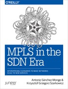
Figure 10-1 provides a simplified view of the forwarding plane inside a multicomponent router, or switch, or firewall, and so on.

Figure 10-1. Single-chassis multiforwarder network device—forwarding plane
The forwarding plane of a multicomponent network device is composed of three types of elements:
- Forwarding engines
- These handle traffic coming from and going out to the outside world. They are responsible for route/label/flow lookup and for all the externally visible forwarding-plane features: packet header manipulation, classification, scheduling, policing, rewrite, replication, filtering, accounting, fine-grained traffic steering, mirroring, sampling, unicast and multicast RPF checks, class-based forwarding, and many others. A line card typically contains one or more forwarders, which in turn are composed of one or more application-specific integrated circuits (ASICs) and/or network processors. The generic term forwarding engine is like an umbrella for many different vendor-specific terms. For example, Juniper calls it a Packet Forwarding Engine (PFE), and Cisco uses different names for each platform: CRS have Packet Switching Engines (PSE) and ASR has Network Processing Units (NPU). Actually, the latter name is also used by Juniper for certain packet processors, too. For simplicity, let’s use the shorter term forwarder to designate a forwarding engine.
- The fabric
- A network device can scale up by using more powerful forwarders, which are typically shipped in newer generation line cards. It also can scale out by having more forwarders. When a device has multiple forwarders, it needs a fabric to interconnect them. Fabrics are much simpler than forwarders: they just know how to move data units from an ingress/source forwarder to an egress/destination forwarder. Conceptually, fabric chips are similar to Asynchronous Transfer Mode (ATM)—or, why not, MPLS—switches that implement a full mesh of virtual circuits among all the forwarders in a given device; their forwarding state contains just a few destinations.
- Links
- Like in any network, the device’s components are linked together. In this example, the physical connections are instantiated via high-speed links at the midplane: don’t look for the cables!
What does this have to do with real networks and with data centers? Well, this internal network has feature-rich edge components (the forwarding engines) and simple core components (the fabric). Now we are talking! Let’s move on with the analogy.
Suppose that the forwarder FWD_0 in Figure 10-1 receives a packet from the outside world. FWD_0 looks at the packet headers and performs a lookup whose result is: send the packet out of port X that is anchored to FWD_2. FWD_0 adds a new header to the packet—which may be previously fragmented, but that’s another story. This header simply says, take me to FWD_2. Then, it sends the packet to the fabric, using a load-balancing algorithm to distribute the data across the fabric chips (FAB_0, FAB_1 up to FAB_X).
Thanks to this extra (tunnel) header, the fabric can switch the packet to FWD_2 without looking at the packet’s content. When it receives the packet from the fabric, FWD_2 removes the extra header and forwards the packet out of port X toward its destination.
Wait, isn’t this tunneling? Indeed, it is tunneling inside the router! True, this tunneling is transparent to the outside world. But packets can flow inside a multicomponent network device, simply because the edge components (forwarders) use an overlay based on a tunneling header that steers the packets through the fabric underlay.
Forwarding engines inside a network device use an overlay to exchange packets with one another. The fabric acts like a dummy underlay. Fabric chips are not capable of doing a real forwarding lookup: they need a header that points to a destination forwarder.
Single-Chassis Network Devices—Control Plane
As in the case of the forwarding plane, let’s use the powerful analogy between a multicomponent single-chassis network device and a multidevice network.
Remember that there are two networks inside a network device: the forwarding plane and the control plane. It’s time to have a look inside the control plane.
Although the general architecture is similar for all vendors, the details of the following example are inspired on a Juniper MX—for example, not all vendors use a TCP/IP stack for the internal control plane.
Figure 10-2 represents one single MX chassis. Rectangular components act like hosts from the point of view of the control plane’s internal network. The Ethernet Bridges, represented with rounded corners, switch internal and external control packets as described here:
-
Internal control packets are natively exchanged between internal hosts through the internal Ethernet Bridges.
-
External control packets are actually coming from, or destined to, the outside world. When a Controller processes external control packets, these are tunneled through the Ethernet Bridges between the Controller and the Control Agent(s).
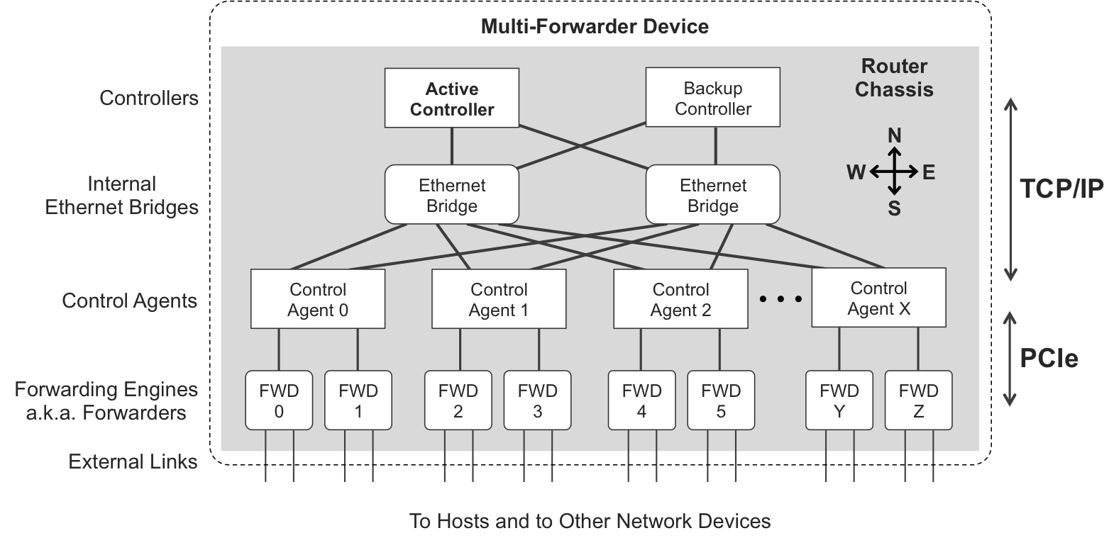
Figure 10-2. Internal control plane in a Juniper MX
Note
At first sight, this topology might remind you of a fabric, but it is not. The topmost elements in a fabric are (spine) switches. Here, they are hosts. And control-plane links have a lower bandwidth than fabric links.
Controller is a generic term for the software that computes all the forwarding rules of the device. This software typically runs on a pair of boards—active and backup—with varied vendor-specific names such as Juniper Routing Engine (RE), Cisco CRS Route Processor (RP), or Cisco ASR Route Switch Processor (RSP). These boards contain multipurpose CPUs that execute the Controller code. Among their many tasks, Controllers are responsible for pushing a forwarding table to Control Agents.
Tip
Junos uses the term Master as an equivalent to Active in an Active-Backup control plane. This is a horizontal relationship. In this book, the term Master is reserved for a different concept: a hierarchical relationship between two Controllers.
Control Agents are also pieces of software that run in less powerful CPUs, typically located in line cards. These are responsible, among other tasks, for translating the high-level instructions received from Controllers into low-level hardware-specific instructions that are optimized and adapted to forwarding ASICs.
Note
Software? Yes, this type of (internal) Networking is also Software-Defined!
Single-chassis network devices—internal control traffic
For the Controllers to send instructions to Control Agents, and for the Control Agents to report events and statistics to Controllers, they need a communication infrastructure: indeed, internal Ethernet Bridges that physically interconnect them.
Every internal host has a MAC address (derived from its physical location) and an IPv4 address. For example, in Junos, the master RE has IPv4 address 128.0.0.1 and line cards have IPv4 address 128.0.0.16+<slot_number>. These addresses reside in a hidden private routing table called __juniper_private1__, whose purpose is to exchange data between Controllers and Control Agents (and also between the Active and Backup Controllers). These addresses are not visible from the outside.
When a Control Agent boots, it gets from the Active Controller via BOOTP (over UDP) both an IPv4 address and the name of the software image, and then it gets the image itself via TFTP (over UDP). After booting, Control Agents establish TCP sessions with Controllers. Controllers use these sessions to send a forwarding table, filter attachments and definitions, class of service structures, and so on to the Control Agents. On the other hand, Control Agents send events and statistics to Controllers via these TCP sessions, too.
Finally, Control Agents adapt the forwarding instruction set to a format that is understandable by the Forwarding Engine ASICs. This is typically a complex layered process with two main stages: a hardware-agnostic stage called Hardware Adaptation Layer (HAL) in Junos, and a hardware-specific layer that depends on the actual chipset in the Forwarding Engine. The resulting microcode instructions and structures are programmed into the ASICs by using a mechanism such as Peripheral Component Interconnect Express (PCIe). Chapter 12 compares this architecture—based on purpose-built ASICs that have a special instruction set used for networking—with the multipurpose x86 architecture, for which only the software (OS or controller) knows that this is a networking device, but the hardware is “dumb.”
Single-chassis multiforwarder devices—external control traffic
So far, we have very briefly seen how the internal control plane works. But a network device needs to exchange control packets with the outside world, too. If a router does not learn routes from the outside, it cannot even compute a useful forwarding table!
Figure 10-3 shows how two adjacent MX routers (CE1 and PE1) exchange an eBGP update. The gray header fields only live in the internal control network, so they cannot be captured with an inline sniffer at the CE1-PE1 link. As for the external MAC header MAC_A→MAC_B, it is surrounded by a dotted line in the internal path because it is not always present. For example, in MX, CE1’s Active Controller builds the packet with that header, which goes on the wire, and PE1 strips the header before sending the packet up to its local Active Controller.

Figure 10-3. Distributed control plane between two Juniper MX devices
It is important to note that the control plane relies on the forwarding plane. Let’s focus on the most interesting aspect: the ingress path at PE1. When the packet arrives to FWD_Y at PE1, a route lookup occurs. The result of this lookup is: the destination is a local IPv4 address; send it up to the control plane. So, the Forwarding Engine hands the packet to the Control Agent on which it depends. The Control Agent adds a Generic Routing Encapsulation (GRE)-like header (the actual protocol used in Juniper devices is called TTP, but it is very similar to GRE).
The resulting packet has two IPv4 headers:
-
An external IPv4 header, from the Control Agent at line card slot #2 (128.0.0.18 = 128.0.0.16+<slot_number>) to the Active Controller (128.0.0.1). Thanks to this header, the packet arrives to PE1’s Active Controller, which removes the tunneling headers and processes the original BGP (CE1→PE1) packet.
-
An internal IPv4 header with the configured—externally visible—addresses at the CE1-PE1 link (10.1.0.0 → 10.1.0.1).
The model represented in Figure 10-3 also applies to the exchange of other one-hop control packets like those used by link-state protocols (OSPF, IS-IS, etc.).
Things become a bit more interesting when the control packet follows an external multihop path, such as that shown in Figure 10-4. Although the examples in previous chapters included a Route Reflector (RR), this implies a hierarchy that makes things more confusing for an initial multihop example. So let’s consider a flat multihop iBGP session between PE1 and PE3 loopback addresses. The original physical interfaces started with ge-2/0/x, so they all belonged to the same forwarder. These numbers have been changed in order to make the example more interesting.
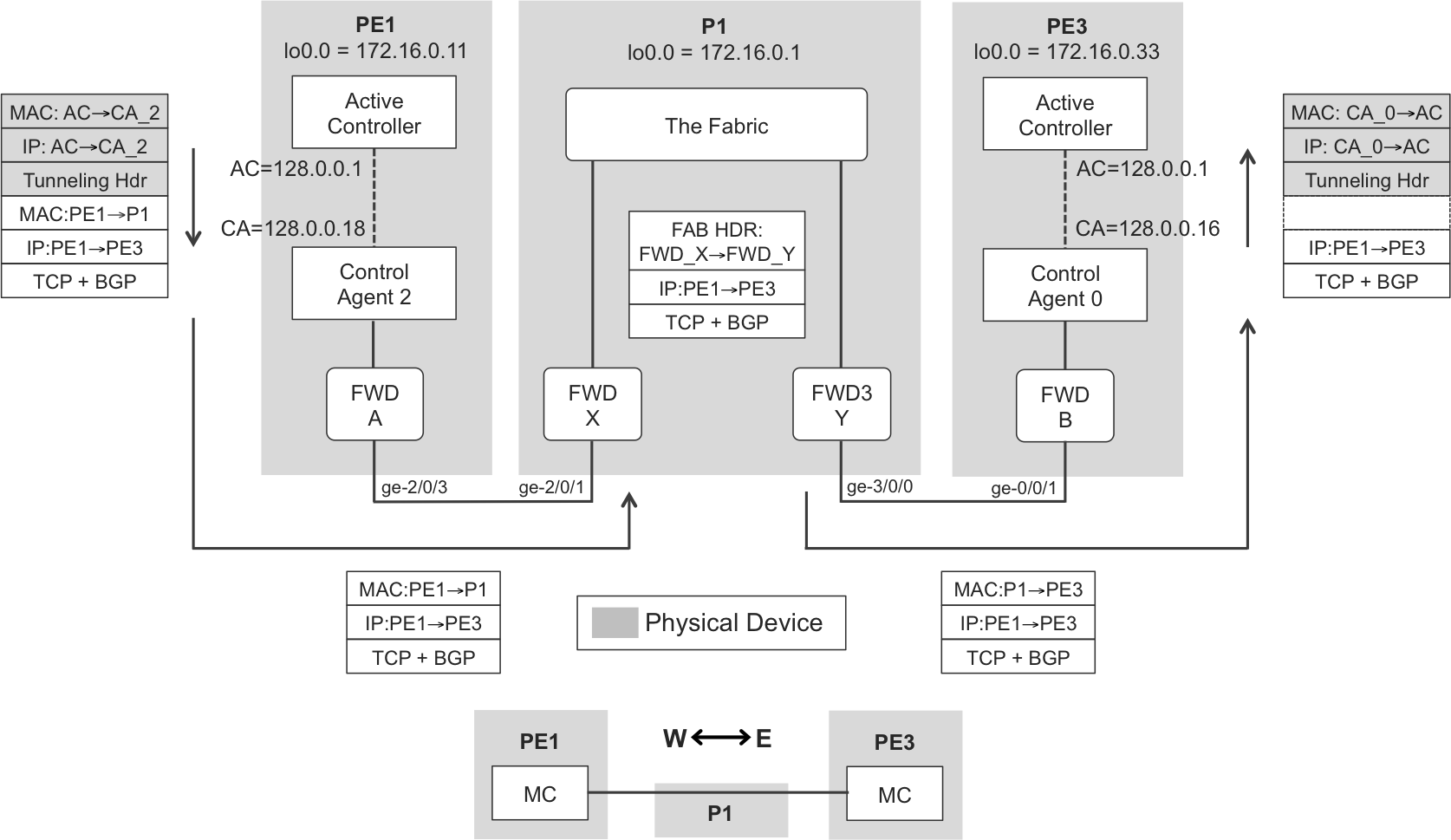
Figure 10-4. Distributed multihop control plane—Juniper MX
From the point of view of P1, the PE1→PE3 iBGP update is not a control packet; it is a transit packet. This raises an important paradigm of modern networking:
-
The control plane does not process the vast majority of the packets that transit a network device. Instead, transit traffic typically uses the high-speed links of the forwarding plane.
-
Only control and exception packets (e.g., IPv4 packets with an expired Time-to-Live [TTL], or with options in their headers) are “punted” to the control plane, bypassing the fabric. The gates between both worlds are the medium-speed links between Control Agents and Forwarders.
Note
Even if an internal Ethernet Bridge may coexist in the same physical cards with Fabric Chips, they are all different functional components. Internal Ethernet Bridges are not part of the fabric.
When P1 receives the BGP update, it does not find anything exceptional: TTL is fine, no IP options, and the destination is out of FWD_Y. So, the packet bypasses the control plane. There are at least a couple of scenarios in which things would have been different:
-
If the packet had TTL expired due to IP forwarding. After passing a hierarchical anti-DDoS rate limiter, the packet reaches the Control Agent. This, in turn, generates an ICMP message back to the original packet’s source informing of the TTL expired condition. The Controller is not bothered for simple tasks like this one.
-
If the packet had IP Options. This would be the case of a non-bundled RSVP PE1→PE3 packet. Even though the destination IP address of such packets is the remote PE, they need to be fully processed, hop by hop, involving all the Active Controllers in the path. As a result, these packets typically do not transit the fabric.
As you can see, a simple PE1→PE3 BGP packet actually undergoes three stages of tunneling: two at internal control-plane networks (PE1 and PE3) and one at a forwarding-plane internal network (P1). This example is adequate to illustrate the relativity of the overlay and underlay concepts. P1 is an underlay from the point of view of the PE1→PE3 BGP update. But P1’s forwarding plane is an overlay built over its underlying fabric.
A very important piece of Figure 10-4 is the simplified diagram at the bottom. Despite all the internal complexity, PE1 and PE3 establish a West-East control peering for which all the internal and external forwarding components are simply an underlay. Many of this chapter’s figures use such an abstraction. Although it is essential to understand the details, there is no need to recall them over and over.
Multichassis Network Devices
One way to scale the forwarding plane of a network device is to use a single control plane to manage several chassis at the same time. The result is often called a virtual chassis. It is virtualization by fusion (several physical devices become one virtual device) rather than fission (one physical server runs several virtual machines [VMs], or one router instantiates several VRFs).
Here is one possible coarse classification of virtual-chassis architectures, from the point of view of the forwarding plane:
-
The fabric is implemented by certain physical devices whose forwarding plane only performs this function. These are dedicated chassis with fabric-only links. They look different and, in fact, are different from the line-card chassis that contain both the forwarding engines and the external facing interfaces. This architecture is beyond the scope of this book.
-
The fabric is implemented by physical devices that could be used as standalone network devices, as well. This architecture will be discussed later.
Let’s zoom out for a moment and take a broader look at data centers. The analogy between multiforwarder (or multichassis) devices and data center networks will naturally unfold.
Legacy Data Center Networking
The previous discussion provides very powerful analogies to data center networking. But it’s important to provide some context before explaining the analogies.
The Challenges of L2 Bridged Networks
In the early days of the Internet, public and private data centers consisted of physical servers connected to legacy L2 bridged networks. And this is still the case in many small and medium-sized data centers and countless private enterprise networks.
Over time, compute virtualization has become more and more popular with the universal adoption of applications running on VMs or containers. There’s no doubt: virtualization is cool, but in the legacy L2 connectivity model, hypervisors are still connected via VLAN trunks to the physical underlay. This takes a huge toll.
Revolution against the VLAN tyranny
In a legacy L2 bridged network, traffic segmentation is achieved by VLANs. Every time that a new server is deployed, its Network Interface Cards (NICs) typically obtain static or dynamic IP addresses. These addresses cannot be freely assigned; they belong to IP subnets, which in turn are rigidly coupled to VLANs. These VLANs must be provisioned all the way from the server (or hypervisor) through the broadcast domain—spanning L2 bridges—to all the host and router interfaces in the VLAN. The result is a monolithic paradigm in which the service and the applications are intimately associated to the network underlay. Despite all the possible attempts to automate and orchestrate this process, in practice the IT staff must coordinate service deployment with the network team; this clearly interferes with business agility.
VLANs were initially proposed as a broadcast containment mechanism. The NICs for end systems are in promiscuous mode for broadcast, so the system performance would be much more affected by broadcasts without VLANs.
Then, the VLAN became a service delimiter mechanism: department isolation, service A versus service B, or customer 1, 2, 3.
As a result, the VLAN tag has two interpretations:
-
It is a (multipoint) circuit identifier at the L2 network infrastructure level.
-
It is a multiplexer for edge devices (hosts, hypervisors, and routers); at the edge, a VLAN is conceptually linked to an L3 network, and it acts like a tenant or a service identifier.
Divide and conquer is a general rule for workable solutions, and a VLAN means too many things. In contrast, modern data center architectures completely decouple the service from the transport; regardless of whether the multiplexing object is an MPLS service label, or a Virtual eXtensible LAN (VXLAN) Network Identifier (VNI), or something else, it is only meaningful for edge devices.
Note
Edge devices in a modern data center must use a multiplexing technique that is decoupled from the underlying infrastructure. In other words, they must use an overlay.
One additional limitation imposed by VLANs is the creation of deployment silos. Imagine that the data center network is composed of an L3 core interconnecting L2 islands. If a legacy application requires L2 connectivity, the application is constrained to just one island. The introduction of an overlay breaks this barrier by allowing any-to-any connectivity.
Oh, yes, and the VLAN ID is just a 12-bit field, so only 4,095 values are available. This is often mentioned as the main reason to use an overlay instead of VLANs. Although it is an important point indeed, there are more compelling reasons to move away from VLANs.
Bandwidth scaling
As mentioned earlier, there are two ways to grow a network: scale up and scale out.
The scale-up approach is limited and very often must be combined with scale out. On the other hand, more network devices and links typically results in a meshed topology full of loops. With an L2 bridged underlay, this is a no-go: Spanning Tree would block most of the redundant links, resulting in a degraded topology. This is one of the main reasons why the underlay in a modern data center must be L3.
Control-plane scaling
L2 bridges typically have a limit on the number of MAC addresses that they can learn—when this limit is reached, the bridge floods frames destined for the new MAC addresses. Core bridges need to learn all the MACs, and this creates a serious scalability issue.
If in order to ease provisioning you configure all the VLANs on hypervisor ports, broadcast significantly loads the control plane in the hypervisor stack.
Network stability and resiliency
Redundant topologies are always looped and, if the underlay is L2 Ethernet, loop avoidance relies on Spanning Tree, which is probably the scariest and most fragile control protocol suite. The broadcast storm beast has been responsible for so many network meltdowns throughout networking history. Simply stated, a broadcast domain is a single point of failure. This is probably the most important reason to claim that L2 bridging is legacy.
Underlays in Modern Data Centers
In a data center, the underlay is a set of interconnected network devices that provide data transport between (physical or virtual) computing systems. You can view this underlay as a core inconnecting edge devices. These edge devices—called here edge forwarders or VPN forwarders—are functionally equivalent to PEs and are responsible for implementing the overlay.
Due to the numerous challenges that L2 bridged networks face, an underlay in a modern data center must be based on L3, pretty much like an SP core underlay.
Oh, some applications require L2 connectivity? In reality, the majority of the applications work perfectly well over L3 (in multihop connections). Technologies such as VM mobility, which traditionally relied on L2, are beginning to support L3, as well. However, many data centers still run applications that require L2 connectivity. Sometimes, data center administrators might not know what particular application has this requirement, but still they decide to prepare their infrastructure for that eventuality. Anyway, when L2 connectivity is needed, it is handled by the overlay. The underlay can definitely remain L3:
-
Network devices build an IP core that is typically modeled as an IP fabric (soon to be explained). IP control plane provides great resiliency and multipath capabilities.
-
In large-scale data centers, the underlay core typically supports native MPLS transport, because MPLS is the only technology that provides the required level of scaling and features required by the most demanding and scalable data centers. Over time, MPLS may be progressively adopted by lower-scale data centers, too.
Overlays in Modern Data Centers
Depending on the logic implemented by an edge device, the overlay can be L3 or L2 (see Figure 10-5). In an analogy to the concepts already covered in previous chapters, these overlays are similar to L3VPNs or L2VPNs.
Figure 10-5. L3 and L2 overlays
Tip
Remember that this book represents frames following the MPLS convention: the upper label is also the outer label. In X over Y, X is actually represented below Y. The wire is on top of the representation.
There are many types of overlay encapsulations available and implemented.
First, here are three MPLS-over-X flavors that are capable of encapsulating both L2 and L3:
-
MPLS-over-GRE encodes a MPLS packet inside the GRE payload.
-
MPLS-over-UDP encodes a MPLS packet inside the UDP payload. The variable values of the source and destination ports in the UDP header makes it a more suitable solution for hashing and load balancing than the less feature-rich original GRE header. However, as of this writing, most network devices do not yet support it.
-
MPLS-over-MPLS is just MPLS VPN as usual. It requires an MPLS-capable underlay.
Next, here are some examples of IP-over-IP tunnels with a multiplexing header:
-
VXLAN is similar to MPLS-over-UDP except that the MPLS label is replaced with a field that gets a different name (VXLAN Network Identifier [VNI]). As of this writing, it is only capable of encapsulating L2 frames because it lacks a control plane for L3.
-
Network Virtualization using GRE (NVGRE) is similar to VXLAN, just that it uses an enhanced GRE header with a multiplexing key instead of VXLAN over UDP. The principle is the same. This is not covered in this book.
-
STT (Stateless Transport Tunneling) uses a TCP-like header but it does not use the TCP logic: it is stateless. The only advantage is the possibility to reuse the TCP offload implementations in host operating system (OS) kernels. This, too, is not covered in this book.
-
Other encapsulations such as Geneve, IEEE 802.1BR, and the next one round the corner.
The actual encapsulation is an implementation detail. What matters are the structural model, the control plane, and the possibility of stacking. From an efficiency perspective, nothing beats a 4-byte stackable header like MPLS. Other overlay encapsulations are available if, for whatever reasons (be they technical or not), MPLS is not desired. Anyway, even if the on-the-wire packet does not have any MPLS headers, the structural model of any overlay is still MPLS-like. This is the spinal chord of the MPLS paradigm. Deep innovation comes with new structural models and not with new encapsulations.
Except for MPLS-over-MPLS, all the listed encapsulations work perfectly well over plain IP networks. VXLAN is a widely adopted L2 overlay in small to medium-sized data centers. Conversely, large-scale data centers typically rely on a native MPLS encapsulation with an MPLS-capable kernel network stack at the servers’ OS.
Remember that VXLAN implements the overlay by embedding a VNI in a transport IP tunnel. The VNI is a multiplexer and its role is similar to a service MPLS label. Chapter 8 already covers VXLAN, including its forwarding plane and an example of a control plane (Ethernet VPN [EVPN]).
Note
Multiplexer fields such as MPLS service labels and VNIs are only significant to edge forwarders. They do not create any state in core or IP fabric devices.
Let’s add a cautionary note about L2 overlays: if an application requires L2 connectivity between end systems in geographically distant data centers, it is possible to stretch the L2 overlay across the WAN. This service is known as Data Center Interconnection (DCI), and you can read more about it in Chapter 8. True, stretching L2 overlays across geographical boundaries might be required by legacy applications, but this does not make it a good practice: it is a remedy. The good practice is to reduce as much as possible the scope of L2 broadcast domains. Even L2 overlays have the risk of loops.
Data Center Underlays—Fabrics
IP fabrics (and MPLS fabrics) have become a de facto underlay in modern data centers. These fabrics are typically composed of many network devices. There is a powerful analogy between a multicomponent device and a multidevice network. Many of the challenges (and solutions) proposed for modern multidevice data center underlays were already addressed, in the context of multicomponent devices, by networking vendors. Of course, the momentum created by the evolution of data center networking has certainly opened new horizons and accelerated the development of more powerful paradigms. But the foundations were already there for decades.
Note
High-scale data centers are evolving toward MPLS fabrics. Indeed, their servers implement a lightweight MPLS stack. The architectural IP fabric concepts discussed in this chapter also apply to MPLS fabrics. You can find some simple examples of the latter in Chapter 2 and Chapter 16.
Traffic in data centers has evolved from a model in which the North-South (client-to-server) traffic pattern was dominant into one in which horizontal (West-East) traffic is very relevant. For example, imagine a video provider with a frontend web application that needs to talk to file services and many other applications—like advertising—inside the same data center. Horizontal traffic appears more and more in the full picture.
IP Fabrics—Forwarding Plane
An IP fabric is simply an IP network with a special physical topology that is very adequate to scale out and to accommodate a growing West-East traffic pattern.
Let’s discuss Figure 10-6, in which all the unshaded boxes are separate physical devices. Beginning at the South, there are VMs, containers (labeled CT), bare-metal servers (labeled BM), and legacy hypervisors. These elements are either not capable or not configured to implement an overlay over an IP network.
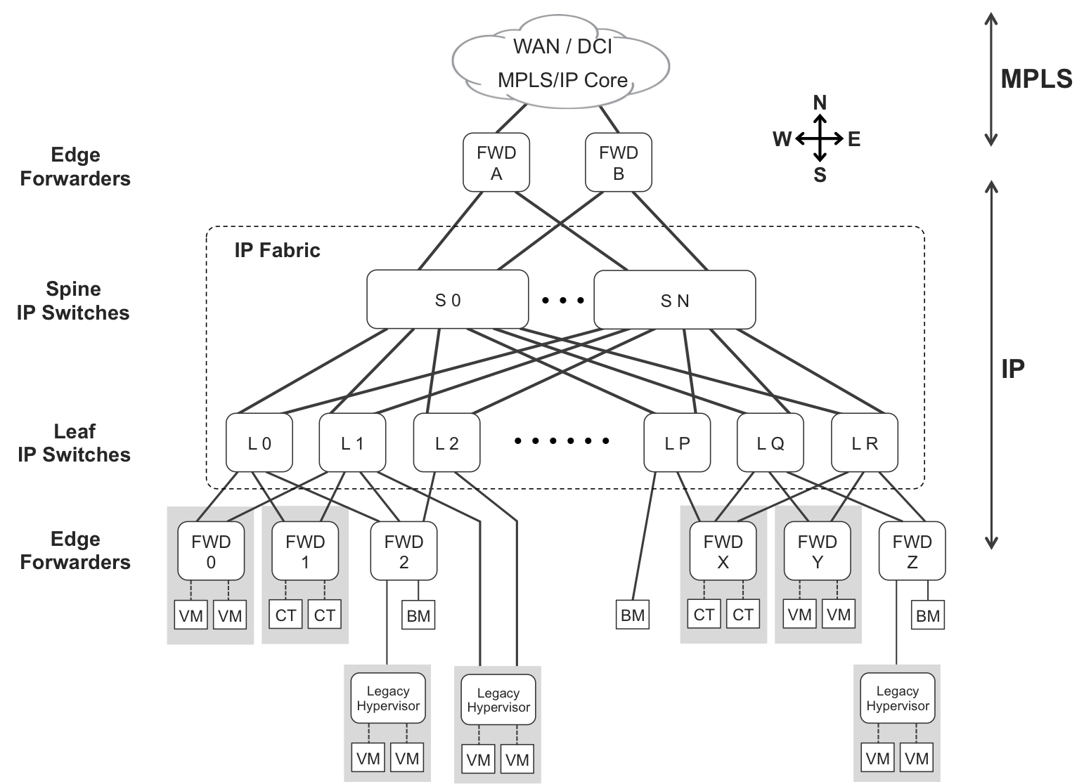
Figure 10-6. Leaf-and-spine architecture—three-stage fabric
Edge forwarders
Edge forwarders (labeled FWD) implement an overlay through the IP Fabric. They are responsible for encapsulating packets or frames coming from their clients—VMs, bare-metal servers, legacy hypervisors, and systems beyond the WAN—into IP tunnels that can be transported through the IP fabric. Likewise, they decapsulate the traffic received from the IP fabric and deliver the resulting data to their clients. Conceptually, they play the same role as do PEs in an SP core.
Note
Don’t look for the term “edge forwarders” in the existing literature. It is a generic term proposed ad hoc in this book to describe that function.
Although this overlay function is typically performed by a dedicated edge forwarder device, optionally it can be performed by a leaf switch, provided that the latter has one or more directly connected hosts that are not overlay-capable.
There are three types of edge forwarders:
-
Modern hypervisors (and host OSs) that implement an overlay stack. In Figure 10-6, these are FWD_0, FWD_1, FWD_X, and FWD_Y. The overlay headers are handled by the forwarder component inside the hypervisor (or host OS). VMs just send and receive plain Ethernet frames: they have no overlay/underlay awareness.
-
Top of the Rack (ToR) switches with an overlay stack, providing connectivity to legacy bare-metal servers and legacy hypervisors which lack an overlay stack. In Figure 10-6, FWD_2 and FWD_Z are dedicated to this function, whereas L_1, L_2, and L_P perform it in combination with their underlay function.
-
PE routers (data center gateways) implementing an overlay stack (FWD_A and FWD_B in Figure 10-6). These gateways typically interconnect the local data center to other data centers (DCI service) and/or to the outside world, represented as the WAN.
Edge forwarders implement an overlay by using an additional set of packet headers, including at least one header that is only meaningful to edge forwarders.
Leaf-and-spine IP switches
The IP fabric spans leaf-and-spine IP switches. These are basically IP routers that transport tunneled traffic, similar to what P-routers do in an IP/MPLS core. The encapsulation in an IP fabric is, obviously, IP! IP switches in a fabric forward the IP packets that are produced by an overlay encapsulation. As for the necessary IP routing logic, it is discussed later in the context of the control plane.
In Figure 10-6, edge forwarders FWD_0, FWD_1, and FWD_2 are multihomed to one or more of these leaf switches: L_0, L_1, and L_2. However, it is not a perfect mesh; for example, FWD_0 and FWD_1 are not connected to L_2. The single bare-metal server connected to L_P is only connected to L_P. The bottom line is that south of the leaf IP switches, there is no connectivity mandate.
Only within the fabric is there such a mandate: each leaf IP switch is connected to every spine IP switch.
Three-stage IP fabrics
In 1952, Charles Clos designed a model for multistage telephone switching systems. Today, this model is still the de facto reference for scale out, nonblocking architectures (you can find more information on Wikipedia). Paraphrasing Yakov Rekhter, one of the fathers of MPLS:
Do not assume that being innovative, or being a technology leader, requires inventing new technologies. To the contrary, one can be quite innovative by simply combining creative use and packaging with high-quality implementation of existing technologies.
The Clos model is being applied over and over to different use cases, always in a very successful manner. Some of them are covered in this chapter.
In Clos terminology:
-
Leaf IP Switches implement fabric stages #1 and #3.
-
Spine IP Switches implement fabric stage #2.
Another frequently used term is Tier. In this topology, spine IP switches are Tier-1, and leaf IP switches are Tier-2. The lower the Tier, the higher is the relevance.
Back to Figure 10-6, let’s suppose that FWD_0 places a user packet inside an IP overlay header whose destination is FWD_Y. Because there is no leaf device connecting FWD_0 to FWD_Y, the packet must go through three stages:
-
Stage 1 via one of the leaf switches connected to FWD_0: L_0 or L_1
-
Stage 2 via one of the spine switches: S_0, S_1, ..., S_N
-
Stage 3 via one of the leaf switches connected to FWD_Y: L_Q or L_R
From the point of view of a packet that flows in the reverse direction, Stage 1 would be on L_Q or L_R, and Stage 3 on L_0 or L_1.
The Clos architecture is a perfect paradigm for optimal bandwidth utilization and, most important, it is typically nonblocking. This means that if you activate two unused ports at Stages 1 and 3, a switching path can be established between them with no impact on the existing paths. In practice, the traffic between a pair of [source forwarder, destination forwarder] can affect the traffic flowing between another pair of forwarders if the links or devices are congested. Of course! However, this congestion is more unlikely with this architecture than with any other. Clos architectures are the best for horizontal scaling.
Five-stage IP fabrics
You can scale-up an IP fabric by making it five-stage. This model is sometimes referred to as multistage (although, strictly speaking, three-stage fabrics are also multistage).
Figure 10-7 illustrates two five-stage fabric topologies in which all the shaded circles are separate physical devices. The Point of Delivery (POD) model is optimized for connect more PODs, in other words, to connect more sites and devices. As for the Performance model, it is perfect for nonblocking scale out. Adding more leaves and more spines efficiently increases the capacity without a major network redesign.
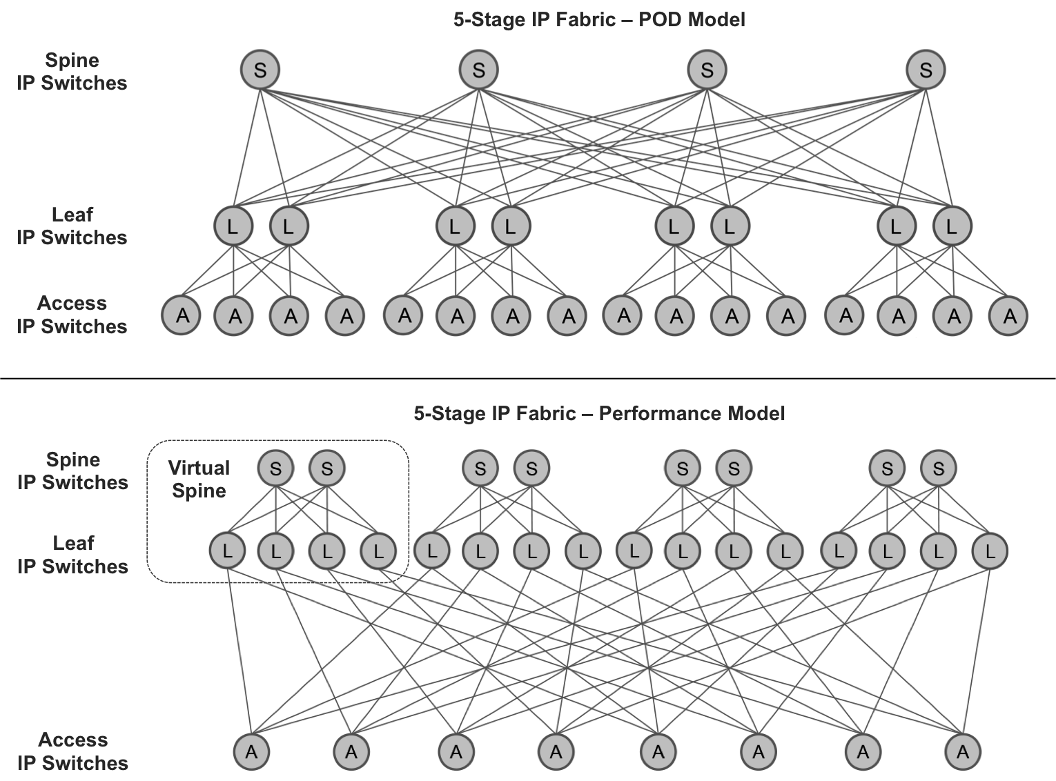
Figure 10-7. Five-stage fabric (courtesy of Doug Hanks)
Warning
There is a practical limit on the number of devices that you can add to any architecture while maintaining the nonblocking property.
Here is the translation from Tier to Stage terminology in the context of five-stage fabrics:
-
Access IP switches are in fabric stages 1 and 5, and are considered Tier-3 devices.
-
Leaf IP switches on Stages 2 and 4 are considered Tier-2 devices.
-
Spine IP switches on Stage 3 are considered Tier-1 devices.
In the POD model, these roles are usually called leaf (stages 1 and 5), spine (stages 2 and 4), and fabric (stage 3).
Another scaling option is to connect IP fabrics with one another on the West-East direction, but this is complex and beyond the scope of this document.
OK, it’s time to talk about the control plane.
IP Fabrics with Distributed-Only Control Plane
For simplicity, let’s discuss a three-stage IP fabric. The concepts for a five-stage IP fabric are exactly the same: just the topology changes.
An IP fabric is composed of network devices that have a forwarding plane. For this reason, Figure 10-8 shows a forwarder component inside each physical device. In this context, the forwarding plane has the role of taking control and transit packets from one device to another. Although not shown for graphical reasons, these packets also traverse the forwarding plane of the leaf IP switches.
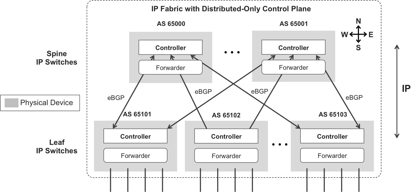
Figure 10-8. IP fabric—distributed-only control plane
You can run any routing protocol between the IP switches, from that of a link-state, to eBGP. A trend in medium and high-scale data centers is to use eBGP because it is simply the most scalable protocol and it has great multipath capabilities. And when the overlay supports native MPLS, this is actually eBGP Labeled Unicast (eBGP-LU), as discussed in Chapter 2 and Chapter 16.
And there is no control plane hierarchy apart from the one imposed by eBGP—spine IP switches readvertise routes from one leaf to another. Nothing fancy in this distributed control plane model: just good-old IP routing as usual.
Figure 10-9 illustrates the forwarding plane in this architecture (for an L3 overlay).
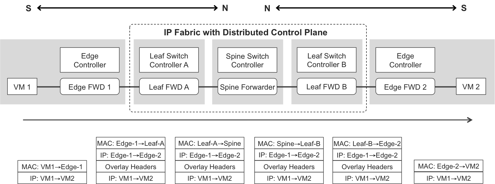
Figure 10-9. Forwarding plane of an IP Fabric with a centralized-only control plane
IP Fabrics with Hybrid Control Plane
It is also possible to have an IP fabric with a hybrid control plane (see Figure 10-10):
-
To perform topology autodiscovery, there is a distributed control plane based on IP routing like the one just described. It is typically a link-state protocol. The goal is to build an internal IP underlay that is able to transport packets between any pair of devices in the fabric.
-
After the topology is discovered, devices can exchange further internal control packets. Through this packet exchange, a spine switch is elected as the active controller of a centralized control plane. Leaf switch controllers are demoted to control agents. Very much like in a multiforwarder single-chassis device, control agents get their forwarding instruction set from the central controller.

Figure 10-10. IP fabric—hybrid control plane
The result is one single virtual device, spanning several physical devices: an enveloped IP fabric. This virtual device is composed of devices that can also run in standalone mode.
IP fabrics have two port types: fabric ports interconnect two IP switches in the fabric, and network ports connect the fabric to the outside world. In a nutshell, the distributed control plane runs on the fabric ports, whereas the centralized control plane programs the network ports.
Having a centralized control plane is useful to program—inside the IP fabric—certain advanced forwarding rules. Enforcing these rules requires acting upon several devices according to a global topology view. For example, the central controller can create automatic link-aggregates at two different levels (next-hop and remote destination), and also build optimized, resilient replication trees for Broadcast, Unknown unicast, and Multicast (BUM).
A centralized IP fabric logic is simple enough to be implemented in the processor of a network device. As an alternative, this logic can also run as an application on an external server or VM.
When its control plane is hybrid, the IP fabric looks like one single device, and as a result, an extra header—the fabric header—steers packets from one leaf to another. The central parts of Figure 10-4 and Figure 10-11 are strictly analogous. In that sense, a leaf IP switch integrated in the IP fabric behaves like a line card, with its control agent and its forwarding engine(s). Figure 10-11 illustrates a L3 overlay example.
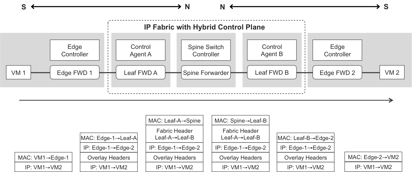
Figure 10-11. Forwarding plane of an IP fabric with a hybrid control plane
Network Virtualization Overlay
As you have just seen, centralizing the control plane of an IP fabric underlay is an interesting option. How about the overlay? At the edge, requirements become more complex: multitenancy, policies, services, and so on. Centralizing the control plane becomes the strongly preferred way to automate the provisioning, evolution, and operation of virtual overlay networks. This is especially true taking into account that there are several types of edge forwarder, and sometimes it is necessary to coordinate all of them to deploy a service. Remember, they can be classified as follows:
-
Hypervisor or Host OS implementing an overlay stack. The overlay header is handled by the forwarder component in the kernel. If the system is virtualized, then VMs or containers just send and receive plain (may be VLAN-tagged) Ethernet frames: they have no awareness of the overlay implementation.
-
ToR switches with an overlay stack, providing connectivity to legacy bare metal servers and hypervisors which lack an overlay stack. These ToR switches act like gateways between the legacy and the overlay worlds.
-
PE routers (data center gateways) implementing an overlay stack.
Modern overlay architectures such as Network Virtualization Overlay (NVO), shown in Figure 10-12, typically have an active-active central control plane that programs the networking stack of overlay-capable hypervisors and host OSs. The resulting architecture is very similar to those in Figure 10-2 and Figure 10-8. Although they need to be interpreted in totally different contexts—a network device, an underlay, and an overlay—they have a common denominator. All of them provide a centralized control plane. There is one way to shape a wheel: round!
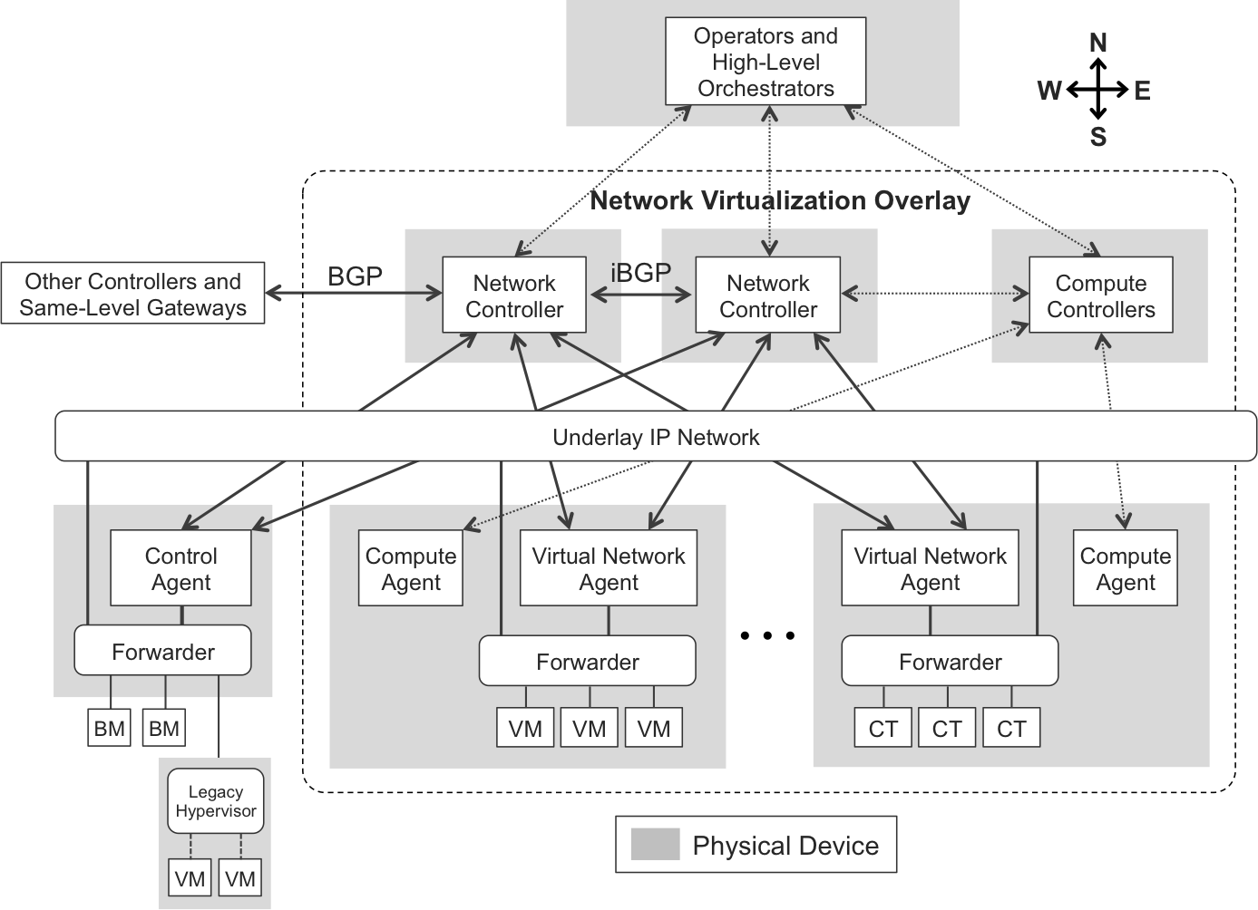
Figure 10-12. NVO control plane
Compute Controllers
To scale-out a virtual compute deployment, it is essential to have a cluster of centralized controllers in charge of defining, instantiating, and moving the virtual computing entities that run on different physical servers.
There are roughly two types of virtual computing entities:
- Virtual machines
- These have their own OS, applications, and libraries. You can see a VM as a full OS with its own kernel running on top a hypervisor. One single hypervisor can run many VMs and provides emulated hardware resources to each VM. Type 1 hypervisors are embedded in the host OS, and Type 2 hypervisors are basically an application that runs on top of yet another host OS. Type 1 hypervisors are more efficient since they involve one less computing layer.
- Containers
- These do not have their own OS. A container is a bundle of applications and dependencies that runs as an isolated process in host OS’ user space. All of the containers running on a given host share the kernel of the host OS.
Both flavors of virtual computing architectures exist in the industry, and there are many different vendor implementations for each of them. As soon as you start adding more physical servers, centralized controllers become handy. Here is an ultra-short list of popular central compute controller examples (there are many more):
-
In the VM world, two different solid references are VMware vCenter and Openstack.
-
In the Container world, Kubernetes (as a centralized controller) and Docker (as a server-local agent and container engine) are popular examples.
Virtual Network Controllers
In legacy compute networking, every virtual interface card in a VM or container is connected to a VLAN. Today, in modern overlay architectures virtual interfaces connect to virtual networks (not VLANs).
Virtual Network Controllers provide a central point of control to define and operate virtual networks together with their policies and forwarding rules.
These controllers typically implement various protocols and programmatic interfaces:
- To the North
- Controllers expose a programmatic northbound interface that an external orchestrator can use to provide an additional level of customized automation to the entire overlay builder solution.
- East-West internal
- Two controllers that belong to the same overlay builder talk to each other through a series of protocols that allow them to synchronize their configuration, state, analytics data, and so on. Among these protocols, there is a special one that performs the function of synchronizing the network overlay routing information. To avoid reinventing the wheel, this protocol can definitely be BGP.
- East-West external
- Controllers can federate to other external controllers via BGP. This provides a good scale-out option by deploying overlay builders in parallel. BGP is also the de facto protocol that controllers use to peer to network gateways.
- To the South
- Controllers send a dynamic forwarding instruction set (networks, policies, etc.) to Control Agents or Virtual Network Agents. Two popular options are XMPP—conceptually, similar to BGP—and OVSDB. These protocols are described later in this book.
Because controllers are the brain that centralizes network signaling, they are also the main entry point for operators and external applications. For this reason, controllers typically expose a GUI, a CLI, a northbound programmatic interface, and so on.
NVO—Transport of Control Packets
Internal Ethernet Bridges in Figure 10-2 are similar to the Underlay IP Network in Figure 10-12, with two main differences:
-
In Figure 10-2, the underlay is L2, whereas in Figure 10-12 it is L3.
-
In Figure 10-2, there is a dedicated control network, whereas in Figure 10-12 control plane packets use the same underlay network that transports transit traffic from the tenants’ applications. This is the typical architecture, although an Out-of-Band control network is an option, too.
NVO—Agents
Virtual Network Agents and Control Agents are responsible for converting the high-level instruction set received from the Controllers into low-level instructions that are adapted and optimized for the forwarders. The name Control Agent is reserved for traditional network devices, whereas Virtual Network Agents run on hypervisors. But they play the same role in the architecture.
In the same way as line cards in a multiforwarder network device, hypervisors are slave entities and they typically implement a very basic user interface as compared to the comprehensive ones offered by the controllers.