3D Transformations
OpenGL has a simple and powerful transformation model. Vertices can be created with position, normal direction, and sets of texture coordinates. These values are manipulated by a series of affine transformations (a linear combinations of translation, rotation, scaling, and shearing) that are set by the application. The fundamental transformation representation in OpenGL is the 4 × 4 matrix. Application-controlled transforms, along with the perspective division functionality available in both positional and texture coordinate pipelines, offer substantial control to the application program. This chapter describes the OpenGL transformation pipeline, providing insights needed to use it effectively, and discusses the transformation issues that can affect visual accuracy.
2.1 Data Representation
Before describing the transformation mechanisms, it is helpful to discuss some details about representations of the transformed data. OpenGL represents vertex coordinates, texture coordinates, normal vectors, and colors generically as tuples. Tuples can be thought of as 4-component vectors. When working with the 1D, 2D, and 3D forms of commands the tuples are implicitly expanded to fill in unspecified components (e.g., for vertex coordinates, an unspecified z coordinate is set to 0 and an unspecified w is set to 1, etc.). OpenGL represents transforms as 4 × 4 matrices, plane equations as 4-component tuples, etc. When thinking about matrix and vector operations on these tuples, it’s helpful to treat them as column vectors, so a point p is transformed by a matrix M by writing it as Mp.
2.2 Overview of the Transformation Pipeline
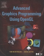
The OpenGL transformation pipeline can be thought of as a series of cartesian coordinate spaces connected by transformations that can be directly set by the application (Figure 2.1). Five spaces are used: object space, which starts with the application’s coordinates, eye space, where the scene is assembled, clip space, which defines the geometry that will be visible in the scene, NDC space, the canonical space resulting from perspective division, and window space, which maps to the framebuffer’s pixel locations. The following sections describe each space in the pipeline, along with its controlling transform, in the order in which they appear in the pipeline.
2.2.1 Object Space and the Modelview Transform
The pipeline begins with texture, vertex, and light position coordinates, along with normal vectors, sent down from the application. These untransformed values are said to be in object space. If the application has enabled the generation of object space texture coordinates, they are created here from untransformed vertex positions.
Object space coordinates are transformed into eye space by transforming them with the current contents of the modelview matrix; it is typically used to assemble a series of objects into a coherent scene viewed from a particular vantage. As suggested by its name, the modelview matrix performs both viewing and modeling transformations.
A modeling transform positions and orients objects in the scene. It transforms all of the primitives comprising an object as a group. In general, each object in the scene may require a different modeling transform to correctly position it. This is done, object by object, by setting the transform then drawing the corresponding objects. To animate an object, its modeling transformation is updated each time the scene is redrawn.
A viewing transform positions and orients the entire collection of objects as a single entity with respect to the “camera position” of the scene. The transformed scene is said to be in eye space. The viewing part of the transformation only changes when the camera position does, typically once per frame.
Since the modelview matrix contains both a viewing transform and a modeling transform, it must be updated when either transform needs to be changed. The modelview matrix is created by multiplying the modeling transform (M) by the viewing transform (V), yielding VM. Typically the application uses OpenGL to do the multiplication of transforms by first loading the viewing transform, then multiplying by a modeling transform. To avoid reloading the viewing transform each time the composite transform needs to be computed, the application can use OpenGL matrix stack operations. The stack can be used to push a copy of the current model matrix or to remove it. To avoid reloading the viewing matrix, the application can load it onto the stack, then duplicate it with a push stack operation before issuing any modeling transforms.
The net result is that modeling transforms are being applied to a copy of the viewing transform. After drawing the corresponding geometry, the composite matrix is popped from the stack, leaving the original viewing matrix on the stack ready for another push, transform, draw, pop sequence.
An important use of the modelview matrix is modifying the parameters of OpenGL light sources. When a light position is issued using the glLight command, the position or direction of the light is transformed by the current modelview matrix before being stored. The transformed position is used in the lighting computations until it’s updated with a new call to glLight. If the position of the light is fixed in the scene (a lamp in a room, for example) then its position must be re-specified each time the viewing transform changes. On the other hand, the light may be fixed relative to the viewpoint (a car’s headlights as seen from the driver’s viewpoint, for example). In this case, the position of the light is specified before a viewing transform is loaded (i.e., while the current transform is the identity matrix).
2.2.2 Eye Space and Projection Transform
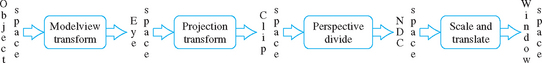
The eye space coordinate system is where object lighting is applied and eye-space texture coordinate generation occurs. OpenGL makes certain assumptions about eye space. The viewer position is defined to be at the origin of the eye-space coordinate system. The direction of view is assumed to be the negative z-axis, and the viewer’s up position is the y-axis (Figure 2.2).
Normals are consumed by the pipeline in eye space. If lighting is enabled, they are used by the lighting equation—along with eye position and light positions–to modify the current vertex color. The projection transform transforms the remaining vertex and texture coordinates into clip space. If the projection transform has perspective elements in it, the w values of the transformed vertices are modified.
2.2.3 Clip Space and Perspective Divide
Clip space is where all objects or parts of objects that are outside the view volume are clipped away, such that
If new vertices are generated as a result of clipping, the new vertices will have texture coordinates and colors interpolated to match the new vertex positions. The exact shape of the view volume depends on the type of projection transform; a perspective transformation results in a frustum (a pyramid with the tip cut off), while an orthographic projection will create a parallelepiped volume.
A perspective divide–dividing the clip space x, y, and z coordinate of each point by its w value–is used to transform the clipped primitives into normalized device coordinate (NDC) space. The effect of a perspective divide on a point depends on whether the clip space w component is 1 or not. If the untransformed positions have a w of one (the common case), the value of w depends on the projection transform. An orthographic transform leaves the w value unmodified; typically the incoming w coordinate is one, so the post-transform w is also one. In this case, the perspective divide has no effect.
A perspective transform scales the w value as a function of the position’s z value; a perspective divide on the resulting point will scale, x y, and z as a function of the untransformed z. This produces the perspective foreshortening effect, where objects become smaller with increasing distance from the viewer. This transform can also produce an undesirable non-linear mapping of z values. The effects of perspective divide on depth buffering and texture coordinate interpolation are discussed in Section 2.8 and Section 6.1.4, respectively.
2.2.4 NDC Space and the Viewport Transform
Normalized device coordinate or NDC space is a screen independent display coordinate system; it encompasses a cube where the x, y, and z components range from −1 to 1. Although clipping to the view volume is specified to happen in clip space, NDC space can be thought of as the space that defines the view volume. The view volume is effectively the result of reversing the divide by wclip operation on the corners of the NDC cube.
The current viewport transform is applied to each vertex coordinate to generate window space coordinates. The viewport transform scales and biases xndc and yndc components to fit within the currently defined viewport, while the zndc component is scaled and biased to the currently defined depth range. By convention, this transformed z value is referred to as depth rather than z. The viewport is defined by integral origin, width, and height values measured in pixels.
2.2.5 Window Space
Window coordinates map primitives to pixel positions in the framebuffer. The integral x and y coordinates correspond to the lower left corner of a corresponding pixel in the window; the z coordinate corresponds to the distance from the viewer into the screen. All z values are retained for visibility testing. Each z coordinate is scaled to fall within the range 0 (closest to the viewer) to 1 (farthest from the viewer), abstracting away the details of depth buffer resolution. The application can modify the z scale and bias so that z values fall within a subset of this range, or reverse the mapping between increasing z distance and increasing depth.
The term screen coordinates is also used to describe this space. The distinction is that screen coordinates are pixel coordinates relative to the entire display screen, while window coordinates are pixel coordinates relative to a window on the screen (assuming a window system is present on the host computer).
2.3 Normal Transformation
OpenGL uses normal vectors for lighting computations and to generate texture coordinates when environment mapping is enabled. Like vertices, normal vectors are transformed from object space to eye space before being used. However, normal vectors are different from vertex positions; they are covectors and are transformed differently (Figure 2.3). Vertex positions are specified in OpenGL as column vectors; normals and some other direction tuples are row vectors. Mathematically, the first is left-multiplied by a matrix, the other has the matrix on the right. If they are both to be transformed the same way (which is commonly done to simplify the implementation code), the matrix must be transposed before being used to transform normals.
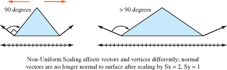
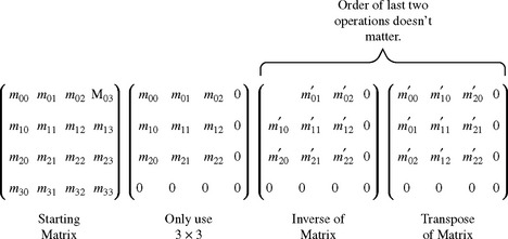
When transforming normals, it’s not enough to simply transpose the matrix. The transform that preserves the relationship between a normal and its surface is created by taking the transpose of the inverse of the modelview matrix (M−1)T, sometimes called the adjoint transpose of M (Figure 2.4). That is, the transformed normal N′ is:
For a “well-behaved” set of transforms consisting of rotations and translations, the resulting modelview matrix is orthonormal.1 In this case, the adjoint transpose of M is M and no work needs to be done.
However, if the modelview matrix contains scaling transforms then more is required. If a single uniform scale s is included in the transform, then M = sI. Therefore M−1 = (1/s)I and the transformed normal vector will be scaled by 1/s, losing its important unit length property (N · N = 1). If the scale factor is non-uniform, then the scale factor computation becomes more complicated (Figure 2.3). If the scaling factor is uniform, and the incoming normals started out with unit lengths, then they can be restored to unit length by enabling GL_RESCALE_NORMAL. This option instructs the OpenGL transformation pipeline to compute s and scale the transformed normal. This is opposed to GL_NORMALIZE, which has OpenGL compute the length of each transformed normal in order to normalize them to unit length. Normalize is more costly, but can handle incoming vectors that aren’t of length one.
2.4 Texture Coordinate Generation and Transformation
Texture coordinates have their own transformation pipeline (Figure 2.5), simpler than the one used for geometry transformations. Coordinates are either provided by the application directly, or generated from vertex coordinates or normal vectors. In either case, the texture coordinates are transformed by a 4 × 4 texture transform matrix. Like vertex coordinates, texture coordinates always have four components, even if only one, two, or three components are specified by the application. The missing components are assigned default values; 0 for s, t, and r values (these coordinates can be thought of as x, y, and z equivalents in texture coordinate space) while the q coordinate (the equivalent of w) is assigned the default value of 1.
2.4.1 Texture Matrix
After being transformed by the texture matrix, the transformed coordinates undergo their own perspective divide, using q to divide the other components. Since texture maps may use anywhere from one to four components, texture coordinate components that aren’t needed to index a texture map are discarded at this stage. The remaining components are scaled and wrapped (or clamped) appropriately before being used to index the texture map. This full 4 × 4 transform with perspective divide applied to the coordinates for 1D or 2D textures will be used as the basis of a number of techniques, such as projected textures (Section 14.9) and volume texturing (Section 20.5.8), described later in the book.
2.4.2 Texture Coordinate Generation
The texture coordinate pipeline can generate texture coordinates that are a function of vertex attributes. This functionality, called texture coordinate generation (texgen), is useful for establishing a relationship between geometry and its associated textures. It can also be used to improve an application’s triangle rate performance, since explicit texture coordinates don’t have to be sent with each vertex. The source (x, y, z, w) values can be untransformed vertices (object space), or vertices transformed by the modelview matrix (eye space).
A great deal of flexibility is available for choosing how vertex coordinates are mapped into texture coordinates. There are several categories of mapping functions in core OpenGL; two forms of linear mapping, a version based on vertex normals, and two based on reflection vectors (the last two are used in environment mapping). Linear mapping generates each texture coordinate from the dot product of the vertex and an application-supplied coefficient vector (which can be thought of as a plane equation). Normal mapping copies the vertex normal vector components to s, t, and r. Reflection mapping computes the reflection vector based on the eye position and the vertex and its normal, assigning the vector components to texture coordinates. Sphere mapping also calculates the reflection vector, but then projects it into two dimensions, assigning the result to texture coordinates s and t.
There are two flavors of linear texgen; they differ on where the texture coordinates are computed. Object space linear texgen uses the x, y, z, and w components of untransformed vertices in object space as its source. Eye-space linear texgen uses the positional components of vertices as its source also, but doesn’t use them until after they have been transformed by the modelview matrix.
Textures mapped with object-space linear texgen appear fixed to their objects; eye-space linear textures are fixed relative to the viewpoint and appear fixed in the scene. Object space mappings are typically used to apply textures to the surface of an object to create a specific surface appearance, whereas eye-space mappings are used to apply texturing effects to all or part of the environment containing the object.
One of OpenGL’s more important texture generation modes is environment mapping. Environment mapping derives texture coordinate values from vectors (such as normals or reflection vectors) rather than points. The applied textures simulate effects that are a function of one or more vectors. Examples include specular and diffuse reflections, and specular lighting effects. OpenGL directly supports two forms of environment mapping; sphere mapping and cube mapping. Details on these features and their use are found in Section 5.4.
2.5 Modeling Transforms
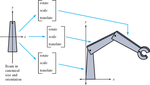
Modeling transforms are used to place objects within the scene. Modeling transforms can position objects, orient them, change their size and shape through scaling and shearing, assemble complex objects by proper placement and orientation of their components, and animate objects by changing these attributes from frame to frame.
Modeling transforms can be thought of as part of an object’s description (Figure 2.6). When an application defines a geometric primitive, it can include modeling transforms to modify the coordinates of the primitive’s vertices. This is useful since it allows re-use of objects. The same object can be used in another part of the scene, with a different size, shape, position, or orientation. This technique can reduce the amount of geometry that the application has to store and send to the graphics pipeline, and can make the modeling process simpler.
Modeling transforms are even more important if an object needs to be animated. A modeling transform can be updated each frame to change the position, orientation, and other properties of an object, animating it without requiring the application to compute and generate new vertex positions each frame. The application can describe a modeling transform parametrically (for example, the angle through which a wheel should be rotated), update the parameter appropriately each frame, then generate a new transform from the parametric description. Note that generating a new transform each frame is generally better than incrementally updating a particular transformation, since the latter approach can lead to large accumulation of arithmetic errors over time.
2.6 Visualizing Transform Sequences
Using transformations to build complex objects from simpler ones, then placing and orienting them in the scene can result in long sequences of transformations concatenated together. Taking full advantage of transform functionality requires being able to understand and accurately visualize the effect of transform combinations.
There are a number of ways to visualize a transformation sequence. The most basic paradigm is the mathematical one. Each transformation is represented as a 4 × 4 matrix. A vertex is represented as a 4 × 1 column vector. When a vertex is sent through the transformation pipeline, the vertex components are transformed by multiplying the column vector v by the current transformation M, resulting in a modified vector v? that is equal to Mv. An OpenGL command stream is composed of updates to the transformation matrix, followed by a sequence of vertices that are modified by the current transform. This process alternates back and forth until the entire scene is rendered.
Instead of applying a single transformation to each vertex, a sequence of transformations can be created and combined into a single 4 × 4 matrix. An ordered set of matrices, representing the desired transform sequence, is multiplied together, and the result is multiplied with the vertices to be transformed. OpenGL provides applications with the means to multiply a new matrix into the current one, growing a sequence of transformations one by one.
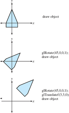
In OpenGL, adding a matrix to a sequence means right multiplying the new matrix with the current transformation. If the current transformation is matrix C, and the new matrix is N, the result of applying the matrix will be a new matrix containing CN. The matrices can be thought of acting from right to left: matrix N can be thought of as acting on the vertex before matrix C. If the sequence of transforms should act in the order A, then B, then C, they should be concatenated together as CBA, and issued to OpenGL in the order C, then B, then A (Figure 2.7).
2.7 Projection Transform
The projection transform establishes which part of the modeled scene will be visible, and what sort of projection will be applied. Although any transformation that can be represented with a 4×4 matrix and a perspective divide can be modeled, most applications will use either a parallel (orthographic) or a perspective projection (Figure 2.8).
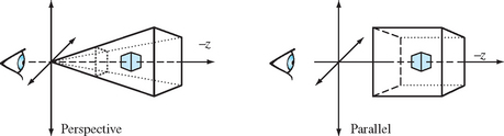
The view volume of a parallel projection is parallelepiped (box shape). The viewer position establishes the front and back of the viewing volume by setting the front and back clipping planes. Objects both in front of and behind the viewer will be visible, as long as they are within the view volume. The glOrtho command establishes a parallel projection, or alternatively, a sequence of translations and scales can be concatenated directly by the application.
A perspective projection changes the value of vertex coordinates being transformed, so the perspective divide step will modify the vertex x, y, and z values. As mentioned in the viewing section, the view volume is now a frustum (truncated pyramid), and the view position relative to the objects in the scene is very important. The degree to which the sides of the frustum diverge will determine how quickly objects change in size as a function of their z coordinate. This translates into a more “wide angle” or “telephoto” view.
2.8 The Z Coordinate and Perspective Projection
The depth buffer is used to determine which portions of objects are visible within the scene. When two objects cover the same x and y positions but have different z values, the depth buffer ensures that only the closer object is visible.
Depth buffering can fail to resolve objects whose z values are nearly the same value. Since the depth buffer stores z values with limited precision, z values are rounded as they are stored. The z values may round to the same number, causing depth buffering artifacts.
Since the application can exactly specify the desired perspective transformation, it can specify transforms that maximize the performance of the depth buffer. This can reduce the chance of depth buffer artifacts. For example, if the glFrustum call is used to set the perspective transform, the properties of the z values can be tuned by changing the ratio of the near and far clipping planes. This is done by adjusting the near and far parameters of the function. The same can be done with the gluPerspective command, by changing the values of zNear and zFar.
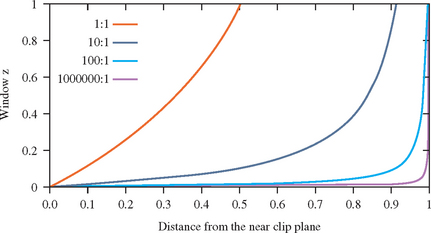
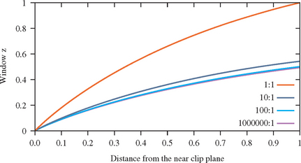
To set these values correctly, it is important to understand the characteristics of the window z coordinate. The z value specifies the distance from the fragment to the plane of the eye. The relationship between distance and z is linear in an orthographic projection, but not in a perspective one. Figure 2.9 plots the window coordinate z value vs. the eye-to-pixel distance for several ratios of far to near. The non-linearity increases the resolution of the z values when they are close to the near clipping plane, increasing the resolving power of the depth buffer, but decreasing the precision throughout the rest of the viewing frustum. As a result, the accuracy of the depth buffer in the back part of the viewing volume is decreased.
For an object a given distance from the eye, however, the depth precision is not as bad as it looks in Figure 2.9. No matter how distant the far clip plane is, at least half of the available depth range is present in the first “unit” of distance. In other words, if the distance from the eye to the near clip plane is one unit, at least half of the z range is used up traveling the same distance from the near clip plane toward the far clip plane. Figure 2.10 plots the z range for the first unit distance for various ranges. With a million to one ratio, the z value is approximately 0.5 at one unit of distance. As long as the data is mostly drawn close to the near plane, the z precision is good. The far plane could be set to infinity without significantly changing the accuracy of the depth buffer near the viewer.
To achieve the best depth buffer precision, the near plane should be moved as far from the eye as possible without touching the object of interest (which would cause part or all of it to be clipped away). The position of the near clipping plane has no effect on the projection of the x and y coordinates, so moving it has only a minimal effect on the image. As a result, readjusting the near plane dynamically shouldn’t cause noticeable artifacts while animating. On the other hand, allowing the near clip plane to be closer to the eye than to the object will result in loss of depth buffer precision.
2.8.1 Z Coordinates and Fog
In addition to depth buffering, the z coordinate is also used for fog computations. Some implementations may perform the fog computation on a per-vertex basis, using the eye-space z value at each vertex, then interpolate the resulting vertex colors. Other implementations may perform fog computations per fragment. In the latter case, the implementation may choose to use the window z coordinate to perform the fog computation. Implementations may also choose to convert the fog computations into a table lookup operation to save computation overhead. This shortcut can lead to difficulties due to the non-linear nature of window z under perspective projections. For example, if the implementation uses a linearly indexed table, large far to near ratios will leave few table entries for the large eye z values. This can cause noticeable Mach bands in fogged scenes.
2.9 Vertex Programs
Vertex programs, sometimes known as “Vertex Shaders”2 provide additional flexibility and programmability to per-vertex operations. OpenGL provides a fixed sequence of operations to perform transform, coordinate generation, lighting and clipping operations on vertex data. This fixed sequence of operations is called the fixed-function pipeline. The OpenGL 1.4 specification includes the ARB_vertex_program extension which provides a restricted programming language for performing these operations and variations on them, sending the results as vertex components to the rest of the pipeline. This programmable functionality is called the programmable pipeline. While vertex programs provide an assembly language like interface, there are also a number of more “C”-like languages. The OpenGL Shading Language3 (GLSL) [KBR03] and Cg [NVI04] are two examples. Vertex programs not only provide much more control and generality when generating vertex position, normal, texture, and color components per-vertex, but also allow micropass sequences to be defined to implement per-vertex shading algorithms.
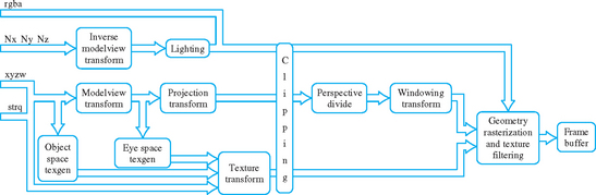
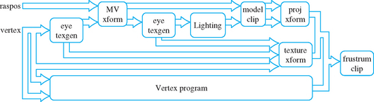
In implementations that support vertex programs, part of the transformation pipeline can be switched between conventional transform mode and vertex program mode. Switching between the two modes is controlled by enabling or disabling the GL_VERTEX_PROGRAM_ARB state value. When enabled, vertex programs bypass the traditional vertex and normal transform functionality, texture coordinate generation and transformation, normal processing (such as renormalization) and lighting, clipping by user-defined clip planes, and per-vertex fog computations. Transform and light extensions, such as vertex weighting and separate specular color, are also replaced by vertex program functionality when it is enabled. Figure 2.11 shows how the two modes are related.
The vertex programming language capabilities are limited to allow efficient hardware implementations: for example, there is no ability to control the flow of the vertex program; it is a linear sequence of commands. The number and type of intermediate results and input and output parameters are also strictly defined and limited. Nevertheless, vertex programming provides a powerful tool further augmenting OpenGL’s use as a graphics assembly language.
2.10 Summary
This chapter only provides an overview of vertex, normal, and texture coordinate transformations and related OpenGL functionality. There are a number of texts that go into these topics in significantly more depth. Beyond the classic computer graphics texts such as that by Foley et al. (1990), there a number of more specialized texts that focus on transformation topics, as well as many excellent linear algebra texts.