In this chapter, we begin our exploration of machine learning models and techniques. The ultimate objective of machine learning is to generalize the facts from some empirical sample data. This is called generalization, and is essentially the ability to use these inferred facts to accurately perform at an accurate rate on new, unseen data. The two broad categories of machine learning are supervised learning and unsupervised learning. The term supervised learning is used to describe the task of machine learning in which an understanding or a model is formulated from some labeled data. By labeled, we mean that the sample data is associated with some observed value. In a basic sense, the model is a statistical description of the data and how the data varies over different parameters. The initial data used by supervised machine learning techniques to create the model is called the training data of the model. On the other hand, unsupervised learning techniques estimate models by finding patterns in unlabeled data. As the data used by unsupervised learning techniques is unlabeled, there is often no definite yes-or-no-based reward system to determine if an estimated model is accurate and correct.
We will now examine linear regression, which is an interesting model that can be used for prediction. As a type of supervised learning, regression models are created from some data in which a number of parameters are somehow combined to produce several target values. The model actually describes the relation between the target value and the model's parameters, and can be used to predict a target value when supplied with the values for the parameters of the model.
We will first study linear regression with single as well as multiple variables, and then describe the algorithms that can be used to formulate machine learning models from some given data. We will study the reasoning behind these models and simultaneously demonstrate how we can implement the algorithms to create these models in Clojure.
We often come across situations where we would need to create an approximate model from some sample data. This model can then be used to predict more such data when its required parameters are supplied. For example, we might want to study the frequency of rainfall on a given day in a particular city, which we will assume varies depending on the humidity on that day. A formulated model could be useful in predicting the possibility of rainfall on a given day if we know the humidity on that day. We start formulating a model from some data by first fitting a straight line (that is, an equation) with some parameters and coefficients over this data. This type of model is called a linear regression model. We can think of linear regression as a way of fitting a straight line, ![]() , over the sample data, if we assume that the sample data has only a single dimension.
, over the sample data, if we assume that the sample data has only a single dimension.
The linear regression model is simply described as a linear equation that represents the regressand or dependent variable of the model. The formulated regression model can have one to several parameters depending on the available data, and these parameters of the model are also termed as regressors, features, or independent variables of the model. We will first explore linear regression models with a single independent variable.
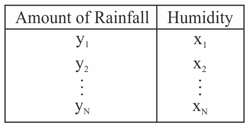
An example problem for using linear regression with a single variable would be to predict the probability of rainfall on a particular day, which depends on the humidity on that day. This training data can be represented in the following tabular form:
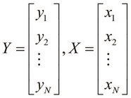
For a single-variable linear model, the dependent variable must vary with respect to a single parameter. Thus, our sample data essentially consists of two vectors, that is, one for the values of the dependent parameter Y and the other for the values of the independent variable X. Both vectors have the same length. This data can be formally represented as two vectors, or single column matrices, as follows:
Let's quickly define the following two matrices in Clojure, X and Y, to represent some sample data:
(def X (cl/matrix [8.401 14.475 13.396 12.127 5.044
                      8.339 15.692 17.108 9.253 12.029]))

(def Y (cl/matrix [-1.57 2.32  0.424  0.814 -2.3
           0.01 1.954 2.296 -0.635 0.328]))
Here, we define 10 points of data; these points can be easily plotted on a scatter graph using the following Incanter scatter-plot function:
(def linear-samp-scatter
  (scatter-plot X Y))

(defn plot-scatter []
  (view linear-samp-scatter))

(plot-scatter)
The preceding code displays the following scatter plot of our data:
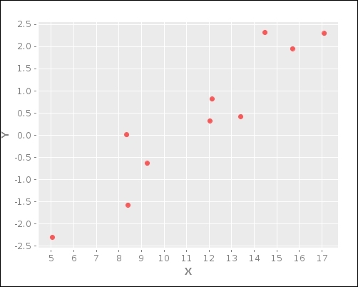
The previous scatter plot is a simple representation of the 10 data points that we defined in X and Y.
Now that we have a visualization of our data, let's estimate a linear model over the given data points. We can generate a linear model of any data using the linear-model function from the Incanter library. This function returns a map that describes the formulated model and also a lot of useful data about this model. For starters, we can plot the linear model over our previous scatter plot by using the :fitted key-value pair from this map. We first get the value of the :fitted key from the returned map and add it to the scatter plot using the add-lines function; this is shown in the following code:
(def samp-linear-model
  (linear-model Y X))
(defn plot-model []
  (view (add-lines samp-scatter-plot
          X (:fitted linear-samp-scatter))))

(plot-model)
This code produces the following self-explanatory plot of the linear model over the scatter plot we defined previously:
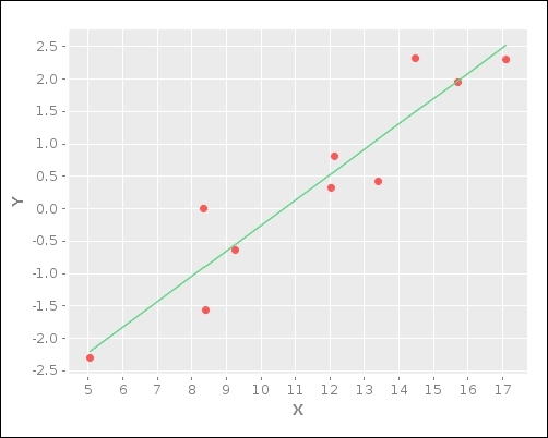
The previous plot depicts the linear model samp-linear-model as a straight line drawn over the 10 data points that we defined in X and Y.
Well, it looks like Incanter's linear-model function did most of the work for us. Essentially, this function creates a linear model of our data by using the ordinary-least squares (OLS) curve-fitting algorithm. We will soon dive into the details of this algorithm, but let's first understand how exactly a curve is fit onto some given data.
Let's first define how a straight line can be represented. In coordinate geometry, a line is simply a function of an independent variable, x, which has a given slope, m, and an intercept, c. The function of the line y can be formally written as ![]() . The slope of the line represents how much the value of y changes when the value of x varies. The intercept of this equation is just where the line meets the y axis of the plot. Note that the equation y is not the same as Y, which actually represents the values of the equation that we have been provided with.
. The slope of the line represents how much the value of y changes when the value of x varies. The intercept of this equation is just where the line meets the y axis of the plot. Note that the equation y is not the same as Y, which actually represents the values of the equation that we have been provided with.
Analogous to this definition of a straight line from coordinate geometry, we formally define the linear regression model with a single variable using our definition of the matrices X and Y, as follows:
This definition of the linear model with a single variable is actually quite versatile since we can use the same equation to define a linear model with multiple variables; we will see this later in the chapter. In the preceding definition, the term ![]() is a coefficient that represents the linear scale of y with respect to x. In terms of geometry, it's simply the slope of a line that fits the given data in matrices X and Y. Since X is a matrix or vector,
is a coefficient that represents the linear scale of y with respect to x. In terms of geometry, it's simply the slope of a line that fits the given data in matrices X and Y. Since X is a matrix or vector, ![]() can also be thought of as a scaling factor for the matrix X.
can also be thought of as a scaling factor for the matrix X.
Also, the term ![]() is another coefficient that explains the value of y when x is zero. In other words, it's the y intercept of the equation. The coefficient
is another coefficient that explains the value of y when x is zero. In other words, it's the y intercept of the equation. The coefficient ![]() of the formulated model is termed as the regression coefficient or effect of the linear model, and the coefficient
of the formulated model is termed as the regression coefficient or effect of the linear model, and the coefficient ![]() is termed as the error term or bias of the model. A model may even have several regression coefficients, as we will see later in this chapter. It turns out that the error
is termed as the error term or bias of the model. A model may even have several regression coefficients, as we will see later in this chapter. It turns out that the error ![]() is actually just another regression coefficient and can be conventionally mentioned along with the other effects of the model. Interestingly, this error determines the scatter or variance of the data in general.
is actually just another regression coefficient and can be conventionally mentioned along with the other effects of the model. Interestingly, this error determines the scatter or variance of the data in general.
Using the map returned by the linear-model function from our earlier example, we can easily inspect the coefficients of the generated model. The returned map has a :coefs key that maps to a vector containing the coefficients of the model. By convention, the error term is also included in this vector, simply as another coefficient:
user> (:coefs samp-linear-model)
[-4.1707801647266045 0.39139682427040384]
Now we've defined a linear model over our data. It's obvious that not all the points will be on a line that is plotted to represent the formulated model. Each data point has some deviation from the linear model's plot over the y axis, and this deviation can be either positive or negative. To represent the overall deviation of the model from the given data, we use the residual sum of squares, mean-squared error, and root mean-squared error functions. The values of these three functions represent a scalar measure of the amount of error in the formulated model.
The difference between the terms error and residual is that an error is a measure of the amount by which an observed value differs from its expected value, while a residual is an estimate of the unobservable statistical error, which is simply not modeled or understood by the statistical model that we are using. We can say that, in a set of observed values, the difference between an observed value and the mean of all values is a residual. The number of residuals in a formulated model must be equal to the number of observed values of the dependent variable in the sample data.
We can use the :residuals keyword to fetch the residuals from the linear model generated by the linear-model function, as shown in the following code:
user> (:residuals samp-linear-model)
[-0.6873445559690581 0.8253111334125092 -0.6483716931997257 0.2383108767994172 -0.10342541689331242 0.9169220471357067 -0.01701880172457293 -0.22923670489146497 -0.08581465024744239 -0.20933223442208365]
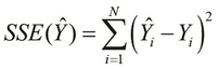
The sum of squared errors of prediction (SSE) is simply the sum of errors in a formulated model. Note that in the following equation, the sign of the error term ![]() isn't significant since we square this difference value; thus, it will always produce a positive value. The SSE is also termed as the residual sum of squares (RSS).
isn't significant since we square this difference value; thus, it will always produce a positive value. The SSE is also termed as the residual sum of squares (RSS).
The linear-model function also calculates the SSE of the formulated model, and this value can be retrieved using the :sse keyword; this is illustrated in the following lines of code:
user> (:sse samp-linear-model)
2.5862250345284887
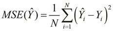
The mean-squared error (MSE) measures the average magnitude of errors in a formulated model without considering the direction of the errors. We can calculate this value by squaring the differences of all the given values of the dependent variable and their corresponding predicted values on the formulated linear model, and calculating the mean of these squared errors. The MSE is also termed as the mean-squared prediction error of a model. If the MSE of a formulated model is zero, then we can say that the model fits the given data perfectly. Of course, this is practically impossible for real data, although we could find a set of values that produce an MSE of zero in theory.
For a given set of N values of the dependent variable ![]() and an estimated set of values
and an estimated set of values ![]() calculated from a formulated model, we can formally represent the MSE function of the formulated model
calculated from a formulated model, we can formally represent the MSE function of the formulated model ![]() as follows:
as follows:
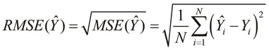
The root mean-squared error (RMSE) or root-mean squared deviation is simply the square root of the MSE and is often used to measure the deviation of a formulated linear model. The RMSE is partial to larger errors, and is hence scale-dependent. This means that the RMSE is particularly useful when large errors are undesirable.
We can formally define the RMSE of a formulated model as follows:
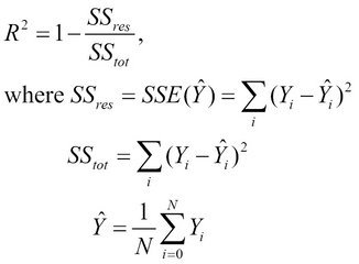
Another measure of the accuracy of a formulated linear model is the coefficient of determination, which is written as ![]() . The coefficient of determination indicates how well the formulated model fits the given sample data, and is defined as follows. This coefficient is defined in terms of the mean of observed values in the sample data
. The coefficient of determination indicates how well the formulated model fits the given sample data, and is defined as follows. This coefficient is defined in terms of the mean of observed values in the sample data ![]() , the SSE, and the total sum of errors
, the SSE, and the total sum of errors ![]() .
.
We can retrieve the calculated value of ![]() from the model generated by the
from the model generated by the linear-model function by using the :r-square keyword as follows:
user> (:r-square samp-linear-model)
0.8837893226172282
In order to formulate a model that best fits the sample data, we should strive to minimize the previously described values. For some given data, we can formulate several models and calculate the total error for each model. This calculated error can then be used to determine which formulated model is the best fit for the data, thus selecting the optimal linear model for the given data.
Based on the MSE of a formulated model, the model is said to have a cost function. The problem of fitting a linear model over some data is equivalent to the problem of minimizing the cost function of a formulated linear model. The cost function, which is represented as ![]() , can be simply thought of as a function of the parameters of a formulated model. Generally, this cost function translates to the MSE of a model. Since the RMSE varies with the formulated parameters of the model, the following cost function of the model is a function of these parameters:
, can be simply thought of as a function of the parameters of a formulated model. Generally, this cost function translates to the MSE of a model. Since the RMSE varies with the formulated parameters of the model, the following cost function of the model is a function of these parameters:
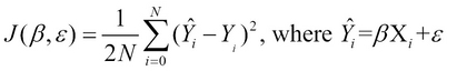
This brings us to the following formal definition of the problem of fitting a linear regression model over some data for the estimated effects ![]() and
and ![]() of a linear model:
of a linear model:
This definition states that we can estimate a linear model, represented by the parameters ![]() and
and ![]() , by determining the values of these parameters, for which the cost function
, by determining the values of these parameters, for which the cost function ![]() takes on the least possible value, ideally zero.
takes on the least possible value, ideally zero.
Let's visualize how the Euclidian space of the cost function of a formulated model varies with respect to the parameters of the model. For this, let's assume that the ![]() parameter that represents the constant error is zero. A plot of the cost function
parameter that represents the constant error is zero. A plot of the cost function ![]() of the linear model over the parameter
of the linear model over the parameter ![]() will ideally appear as a parabolic curve, similar to the following plot:
will ideally appear as a parabolic curve, similar to the following plot:
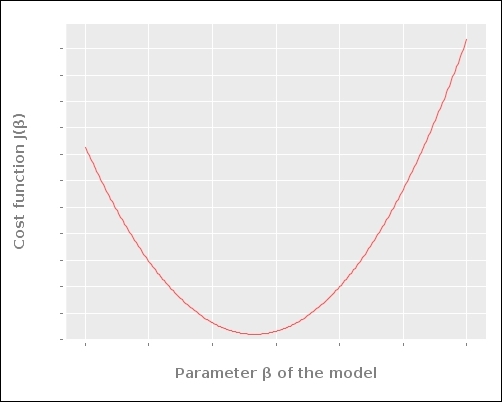
For a single parameter, ![]() , we can plot the preceding chart, which has two dimensions. Similarly, for two parameters,
, we can plot the preceding chart, which has two dimensions. Similarly, for two parameters, ![]() and
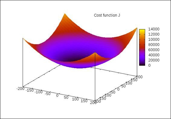
and ![]() , of the formulated model, a plot of three dimensions is produced. This plot appears bowl-shaped or having a convex surface, as illustrated in the following diagram. Also, we can generalize this for N parameters of the formulated model and produce a plot of
, of the formulated model, a plot of three dimensions is produced. This plot appears bowl-shaped or having a convex surface, as illustrated in the following diagram. Also, we can generalize this for N parameters of the formulated model and produce a plot of ![]() dimensions.
dimensions.