The gradient descent algorithm is one of the simplest, although not the most efficient techniques to formulate a linear model that has the least possible value for the cost function or error of the model. This algorithm essentially finds the local minimum of the cost function for a formulated linear model.

As we previously described, a three-dimensional plot of the cost function for a single-variable linear regression model would appear as a convex or bowl-shaped surface with a global minimum. By minimum, we mean that the cost function has the least possible value at this point on the surface of the plot. The gradient descent algorithm essentially starts from any point on the surface and performs a sequence of steps to approach the local minimum of the surface.

This process can be imagined as dropping a ball into a valley or between two adjacent hills, as a result of which the ball slowly rolls towards the point that has the least elevation above sea level. The algorithm is repeated until the value of the apparent cost function from the current point on the surface converges to zero, which figuratively means that the ball rolling down the hill comes to a stop, as we described earlier.

Of course, gradient descent may not really work if there are multiple local minimums on the surface of the plot. However, for an appropriately scaled single-variable linear regression model, the surface of the plot always has a single global minimum, as we illustrated earlier. Thus, we can still use the gradient descent algorithm in such situations to find the global minimum of the surface of the plot.

The gist of this algorithm is that we start from some point on the surface and then take several steps towards the lowest point. We can formally represent this with the following equality:

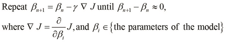
Here, we start from the point represented by on the plot of the cost function J, and incrementally subtract the product of the first-order partial derivative of the cost function , which is derived with respect to the parameters of the formulated model. This means that we slowly step downwards on the surface towards the local minimum, until we cannot find a lower point on the surface. The term determines how large our steps towards the local minimum are, and is called the step of the gradient descent algorithm. We repeat this iteration until the difference between and converges to zero, or at least reduces to a threshold value close to zero.

The process of stepping down towards the local minimum of the surface of the cost functions plot is illustrated in the following diagram:

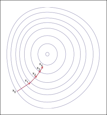
The preceding illustration is a contour diagram of the surface of the plot, in which the circular lines connect the points with an equal height. We start from the point and perform a single iteration of the gradient descent algorithm to step down the surface to point . We repeat this process until we reach the local minimum of the surface with respect to the initial starting point . Note that, through each iteration, the size of the step reduces since the slope of a tangent to this surface also tends to zero as we approach the local minimum.

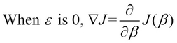
For a single-variable linear regression model with an error constant that is equal to zero, we can simplify the partial derivative component of the gradient descent algorithm. When there is only one parameter of the model, , the first order partial derivate is simply the slope of a tangent at that point on the surface of the plot. Thus, we calculate the slope of this tangent and take a step in the direction of this slope such that we arrive at a point of elevation above the y axis. This is shown in the following formula:

We can implement this simplified version of the gradient descent algorithm as follows:

(def gradient-descent-precision 0.001)

(defn gradient-descent
  "Find the local minimum of the cost function's plot"
  [F' x-start step]
  (loop [x-old x-start]
    (let [x-new (- x-old
                   (* step (F' x-old)))
          dx (- x-new x-old)]
      (if (< dx gradient-descent-precision)
        x-new
        (recur x-new)))))

In the preceding function, we begin from the point x-start and recursively apply the gradient descent algorithm until the value x-new converges. Note that this process is implemented as a tail recursive function using the loop form.

Using partial differentiation, we can formally express how both the parameters and can be calculated using the gradient descent algorithm as follows: