Linear regression estimates some given training data using a linear equation; this solution may not always be the best fit for the given data. Of course, it depends largely on the problem that we are trying to model. Regularization is a commonly used technique to provide a better fit for the data. Generally, a given model is regularized by reducing the effect of some of the independent variables of the model. Alternatively, we could model it as a higher-order polynomial. Regularization isn't exclusive to linear regression, and most machine learning algorithms use some form of regularization in order to create a more accurate model from the given training data.

A model is said to be underfit or high bias when it doesn't estimate the dependent variable to a value that is close to the observed values of the dependent variable in the training data. On the other hand, a model can also be called overfit, or said to have high variance, when the estimated model fits the data perfectly, but isn't general enough to be useful for prediction. Overfit models often describe random errors or noise in the training data instead of the underlying relationship between the dependent and independent variables of the model. The best fit regression model generally lies in between the models created by underfitting and overfitting models and can be obtained through the process of regularization.

A commonly used method for the regularization of an underfit or overfit model is Tikhnov regularization. In statistics, this method is also called ridge regression. We can describe the general form of Tikhnov regularization as follows:

Suppose A represents a mapping from the vector of independent variables x to the dependent variable y. The value A is analogous to the parameter vector of a regression model. The relationship between the vector x and the observed values of the dependent variable, written as b, can be expressed as follows.

An underfit model has a significant error, or rather deviation, with respect to the actual data. We should strive to minimize this error. This can be formally expressed as follows and is based on the sum of residues of the estimated model:

Tikhnov regularization adds a penalized least squares term to the preceding equation to prevent overfitting and is formally defined as follows:

The term in the preceding equation is called the regularization matrix. In the simplest form of Tikhnov regularization, this matrix takes the value , where is a constant. Although applying this equation to a regression model is beyond the scope of this book, we can use Tikhnov regularization to produce a linear regression model with the following cost function:

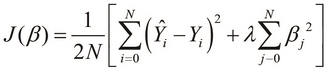
In the preceding equation, the term is called the regularization parameter of the model. This value must be chosen appropriately as larger values for this parameter could produce an underfit model.

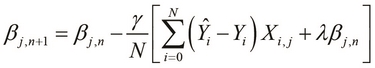
Using the previously defined cost function, we can apply a gradient descent to determine the parameter vector as follows:

We can also apply regularization to the OLS method of determining the parameter vector as follows:

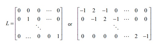
In the preceding equation, L is called the smoothing matrix, and can take on the following forms. Note that we've used the latter form of the definition of L in Chapter 1, Working with Matrices.

Interestingly, when the regularization parameter in the preceding equation is 0, the regularized solution reduces to the original solution using the OLS method.