
We can also use decision trees to model a given classification problem. A decision tree is, in fact, constructed from the given training data, and we can use this decision tree to predict the class of a given set of observed values. The process of constructing a decision tree is loosely based on the concepts of information entropy and information gain from information theory (for more information, refer to Induction of Decision Trees). It is also often termed as decision tree learning. Unfortunately, a detailed study of information theory is beyond the scope of this book. However, in this section, we will explore some concepts in information theory that will be used in the context of machine learning.
A decision tree is a tree or graph that describes a model of decisions and their possible consequences. An internal node in a decision tree represents a decision, or rather a condition of a particular feature in the context of classification. It has two possible outcomes that are represented by the left and right subtrees of the node. Of course, a node in the decision tree could also have more than two subtrees. Each leaf node in a decision tree represents a particular class, or a consequence, in our classification model.
For example, our previous classification problem involving the fish packaging plant could have the following decision tree:
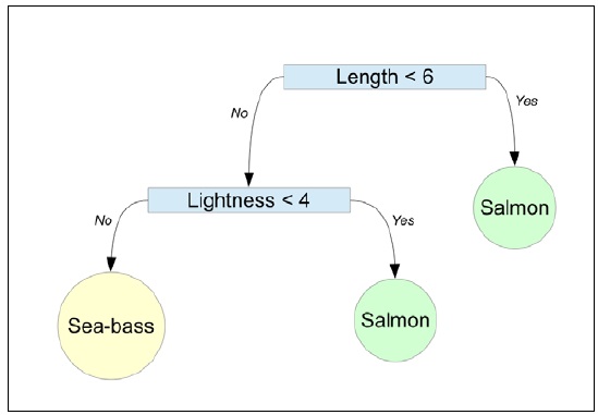
The previously illustrated decision tree uses two conditions to classify a fish as either a salmon or a sea bass. The internal nodes represent the two conditions based on the features of our classification model. Note that the decision tree uses only two of the three features of our classification model. We can thus say the tree is pruned. We shall briefly explore this technique as well in this section.
To classify a set of observed values using a decision tree, we traverse the tree starting from the root node until we reach a leaf node that represents the predicted class of the set of observed values. This technique of predicting the class of a set of observed values from a decision tree is always the same, irrespective of how the decision tree was constructed. For the decision tree described earlier, we can classify a fish by first comparing its length followed by the lightness of its skin. The second comparison is only needed if the length of the fish is greater than 6 as specified by the internal node with the expression Length < 6 in the decision tree. If the length of the fish is indeed greater than 6, we use the lightness of the skin of the fish to decide whether it's a salmon or a sea bass.
There are actually several algorithms that are used to construct a decision tree from some training data. Generally, the tree is constructed by splitting the set of sample values in the training data into smaller subsets based on an attribute value test. The process is repeated on each subset until splitting a given subset of sample values no longer adds internal nodes to the decision tree. As we mentioned earlier, it's possible for an internal node in a decision tree to have more than two subtrees.
We will now explore the C4.5 algorithm to construct a decision tree (for more information, refer to C4.5: Programs for Machine Learning). This algorithm uses the concept of information entropy to decide the feature and the corresponding value on which the set of sample values must be partitioned. Information entropy is defined as the measure of uncertainty in a given feature or random variable (for more information, refer to "A Mathematical Theory of Communication").
For a given feature or attribute f, which has values within the range of 1 to m, we can define the information entropy of the ![]() feature as follows:
feature as follows:
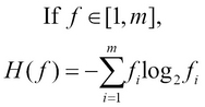
In the preceding equation, the term ![]() represents the number of occurrences of the feature f with respect to the value i. Based on this definition of the information entropy of a feature, we define the normalized information gain
represents the number of occurrences of the feature f with respect to the value i. Based on this definition of the information entropy of a feature, we define the normalized information gain ![]() . In the following equality, the term T refers to the set of sample values or training data supplied to the algorithm:
. In the following equality, the term T refers to the set of sample values or training data supplied to the algorithm:
In terms of information entropy, the preceding definition of the information gain of a given attribute is the change in information entropy of the total set of values when the attribute f is removed from the given set of features in the model.
The algorithm selects a feature A from the given set of features in the training data such that the feature A has the maximum possible information gain in the set of features. We can represent this with the help of the following equality:
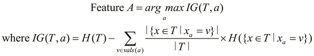
In the preceding equation, ![]() represents the set of all the possible values that a feature a is known to have. The
represents the set of all the possible values that a feature a is known to have. The ![]() set represents the observed values in which the feature a has the value v and the term
set represents the observed values in which the feature a has the value v and the term ![]() represents the information entropy of this set of values.
represents the information entropy of this set of values.
Using the preceding equation to select a feature with the maximum information gain from the training data, we can describe the C4.5 algorithm through the following steps:
- For each feature a, find the normalized information gain from partitioning the sample data on the feature a.
- Select the feature A with the maximum normalized information gain.
- Create an internal decision node based on the selected feature A. Both the subtrees created from this step are either leaf nodes or a new set of sample values to be partitioned further.
- Repeat this process on each partitioned set of sample values produced from the previous step. We repeat the preceding steps until all the features in a subset of sample values have the same information entropy.
Once a decision tree has been created, we can optionally perform pruning on the tree. Pruning is simply the process of removing any extraneous decision nodes from the tree. This can be thought of as a form for the regularization of decision trees through which we prevent underfitting or overfitting of the estimated decision tree model.
J48 is an open source implementation of the C4.5 algorithm in Java, and the clj-ml library contains a working J48 decision tree classifier. We can create a decision tree classifier using the make-classifier function, and we supply the keywords :decision-tree and :c45 as parameters to this function to create a J48 classifier as shown in the following code:
(def DT-classifier (make-classifier :decision-tree :c45))

(defn train-DT-classifier []
  (dataset-set-class fish-dataset 0)
  (classifier-train DT-classifier fish-dataset))
The train-DT-classifier function defined in the preceding code simply trains the classifier represented by DT-classifier with the training data from our previous example of the fish packaging plant. The classifier-train function also prints the following trained classifier:
user> (train-DT-classifier)
#<J48 J48 pruned tree
------------------
width <= 3: sea-bass (2320.0)
width > 3
|   length <= 6
|   |   lightness <= 5: salmon (7147.0/51.0)
|   |   lightness > 5: sea-bass (95.0)
|   length > 6: sea-bass (438.0)

Number of Leaves  : 4

Size of the tree : 7
>
The preceding output gives a good idea of what the decision tree of the trained classifier looks like as well as the size and number of leaf nodes in the decision tree. Apparently, the decision tree has three distinct internal nodes. The root node of the tree is based on the width of a fish, the subsequent node is based on the length of a fish, and the last decision node is based on the lightness of the skin of a fish.
We can now use the decision tree classifier to predict the class of a fish, and we use the following classifier-classify function to perform this classification:
user> (classifier-classify DT-classifier sample-fish)
:salmon
As shown in the preceding code, the classifier predicts the class of the fish represented by sample-fish as a :salmon keyword just like the other classifiers used in the earlier examples.
The J48 decision tree classifier implementation provided by the clj-ml library performs pruning as a final step while training the classifier. We can generate an unpruned tree by specifying the :unpruned key in the map of options passed to the make-classifier function as shown in the following code:
(def UDT-classifier (make-classifier
                     :decision-tree :c45 {:unpruned true}))
The previously defined classifier will not perform pruning on the decision tree generated from training the classifier with the given training data. We can inspect what an unpruned tree looks like by defining and calling the train-UDT-classifier function, which simply trains the classifier using the classifier-train function with the fish-dataset training data. This function can be defined as being analogous to the train-UDT-classifier function and produces the following output when it is called:
user> (train-UDT-classifier)
#<J48 J48 unpruned tree
------------------
width <= 3: sea-bass (2320.0)
width > 3
|   length <= 6
|   |   lightness <= 5
|   |   |   length <= 5: salmon (6073.0)
|   |   |   length > 5
|   |   |   |   width <= 4
|   |   |   |   |   lightness <= 3: salmon (121.0)
|   |   |   |   |   lightness > 3
|   |   |   |   |   |   lightness <= 4: salmon (52.0/25.0)
|   |   |   |   |   |   lightness > 4: sea-bass (50.0/24.0)
|   |   |   |   width > 4: salmon (851.0)
|   |   lightness > 5: sea-bass (95.0)
|   length > 6: sea-bass (438.0)

Number of Leaves  : 8

Size of the tree : 15
As shown in the preceding code, the unpruned decision tree has a lot more internal decision nodes as compared to the decision tree that is generated after pruning it. We can now use the following classifier-classify function to predict the class of a fish using the trained classifier:
user> (classifier-classify UDT-classifier sample-fish)
:salmon
Interestingly, the unpruned tree also predicts the class of the fish represented by sample-fish as :salmon, thus agreeing with the class predicted by the pruned decision tree, which we had described earlier. In summary, the clj-ml library provides us with a working implementation of a decision tree classifier based on the C4.5 algorithm.
The make-classifier function supports several interesting options for the J48 decision tree classifier. We've already explored the :unpruned option, which indicated that the decision tree is not pruned. We can specify the:reduced-error-pruning option to the make-classifier function to force the usage of reduced error pruning (for more information, refer to "Pessimistic decision tree pruning based on tree size"), which is a form of pruning based on reducing the overall error of the model. Another interesting option that we can specify to the make-classifier function is the maximum number of internal nodes or folds that can be removed by pruning the decision tree. We can specify this option using the :pruning-number-of-folds option, and by default, the make-classifier function imposes no such limit while pruning the decision tree. Also, we can specify that each internal decision node in the decision tree has only two subtrees by specifying the :only-binary-splits option to the make-classifier function.