Hierarchical clustering is another method of cluster analysis in which input values from the training data are grouped together into a hierarchy. The process of creating the hierarchy can be done in a top-down approach, where in all observations are first part of a single cluster and are then divided into smaller clusters. Alternatively, we can group the input values using a bottom-up methodology, where each cluster is initially a sample value from the training data and these clusters are then combined together. The former top-down approach is termed as divisive clustering and the later bottom-up method is called agglomerative clustering.

Thus, in agglomerative clustering, we combine clusters into larger clusters, whereas we divide clusters into smaller ones in divisive clustering. In terms of performance, modern implementations of agglomerative clustering algorithms have a time complexity of , while those of divisive clustering have much higher complexity of .

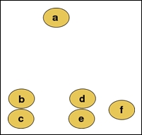
Suppose we have six input values in our training data. In the following illustration, assume that these input values are positioned according to some two-dimensional metric to measure the overall value of a given input value:

We can apply agglomerative clustering on these input values to produce the following hierarchy of clusters:

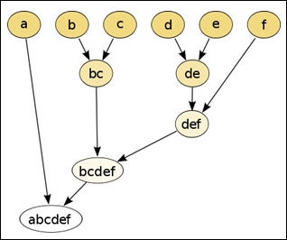
The values b and c are observed to be the closest to each other in the spatial distribution and are hence grouped into a cluster. Similarly, the nodes d and e are also grouped into another cluster. The final result of hierarchically clustering the input value is a single binary tree or a dendogram of the sample values. In effect, clusters such as bc and def are added to the hierarchy as binary subtrees of values or of other clusters. Although this process tends to appear very simple in a two-dimensional space, the solution to the problem of determining the distance and hierarchy between input values is much less trivial when applied over several dimensions of features.

In both agglomerative and divisive clustering techniques, the similarity between input values from the sample data has to be calculated. This can be done by measuring the distance between two sets of input values, grouping them into clusters using the calculated distance, and then determining the linkage or similarity between two clusters of input values.

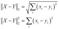
The choice of the distance metric in a hierarchical clustering algorithm will determine the shape of the clusters that are produced by the algorithm. A couple of commonly used measures of the distance between two input vectors and are the Euclidean distance and the squared Euclidean distance , which can be formally expressed as follows:

Another commonly used metric of the distance between input values is the maximum distance , which calculates the maximum absolute difference of corresponding elements in two given vectors. This function can be expressed as follows:

The second aspect of a hierarchical clustering algorithm is the linkage criteria, which is an effective measure of similarity or dissimilarity between two clusters of input values. Two commonly used methods of determining the linkage between two input values are complete linkage clustering and single linkage clustering. Both of these methods are forms of agglomerative clustering.

In agglomerative clustering, two input values or clusters with the shortest distance metric are combined into a new cluster. Of course, the definition of "shortest distance" is what is unique in any agglomerative clustering technique. In complete linkage clustering, input values farthest from each other are used to determine the grouping. Hence, this method is also termed as farthest neighbor clustering. This metric of the distance between two values can be formally expressed as follows:

In the preceding equation, the function is the selected metric of distance between two input vectors. Complete linkage clustering will essentially group together values or clusters that have the maximum value of the distance metric . This operation of grouping together clusters is repeated until a single cluster is produced.

In single linkage clustering, values that are nearest to each other are grouped together. Hence, single linkage clustering is also called nearest neighbor clustering. This can be be formally stated using the following expression:

Another popular hierarchical clustering technique is the Cobweb algorithm. This algorithm is a form of conceptual clustering, in which a concept is created for each cluster produced by the clustering method used. By the term "concept", we mean a concise formal description of the data clustered together. Interestingly, conceptual clustering is closely related to decision tree learning, which we already discussed in Chapter 3, Categorizing Data. The Cobweb algorithm groups all clusters into a classification tree, in which each node contains a formal summary of the values or clusters that are its child nodes. This information can then be used to determine and predict the category of an input value with some missing features. In this sense, this technique can be used when some of the samples in the test data have missing or unknown features.

We now demonstrate a simple implementation of hierarchical clustering. In this implementation, we take a slightly different approach where we embed part of the required functionality into the standard vector data structure provided by the Clojure language.

[org.clojure/math.numeric-tower "0.0.4"]

(ns my-namespace
  (:use [clojure.math.numeric-tower :only [sqrt]]))

For this implementation, we will use the Euclidean distance between two points as a distance metric. We can calculate this distance from the sum of squares of the elements in an input vector, which can be computed using a composition of the reduce and map functions as follows:

(defn sum-of-squares [coll]
  (reduce + (map * coll coll)))

The sum-of-squares function defined in the preceding code will be used to determine the distance metric. We will define two protocols that abstract the operations we perform on a particular data type. From an engineering perspective, these two protocols could be combined into a single protocol, since both the protocols will be used in combination.

However, we use the following two protocols for this example for the sake of clarity:

(defprotocol Each
  (each [v op w]))

(defprotocol Distance
  (distance [v w]))

The each function defined in the Each protocol applies a given operation op on corresponding elements in two collections v and w. The each function is quite similar to the standard map function, but each allows the data type of v to decide how to apply the function op. The distance function defined in the Distance protocol calculates the distance between any two collections v and w. Note that we use the generic term "collection" since we are dealing with abstract protocols and not concrete implementations of the functions of these protocols. For this example, we will implement the preceding protocols as part of the vector data type. Of course, these protocols could also be extended to other data types such as sets and maps.

In this example, we will implement single linkage clustering as the linkage criteria. First, we will have to define a function to determine the two closest vectors from a set of vector values. To do this, we can apply the min-key function, which returns the key with the least associated value in a collection, on a vector. Interestingly, this is possible in Clojure since we can treat a vector as a map with the index values of the various elements in the vector as its keys. We will implement this with the help of the following code:

(defn closest-vectors [vs]
  (let [index-range (range (count vs))]
    (apply min-key
           (fn [[x y]] (distance (vs x) (vs y)))
           (for [i index-range
                 j (filter #(not= i %) index-range)]
             [i j]))))

The closest-vectors function defined in the preceding code determines all possible combinations of the indexes of the vector vs using the for form. Note that the vector vs is a vector of vectors. The distance function is then applied over the values of the possible index combinations and these distances are then compared using the min-key function. The function finally returns the index values of the two inner vector values that have the least distance from each other, thus implementing single linkage clustering.

We will also need to calculate the mean value of two vectors that have to be clustered together. We can implement this using the each function we had previously defined in the Each protocol and the reduce function, as follows:

(defn centroid [& xs]
  (each
   (reduce #(each %1 + %2) xs)
   *
   (double (/ 1 (count xs)))))

The centroid function defined in the preceding code will calculate the mean value of a sequence of vector values. Note the use of the double function to ensure that the value returned by the centroid function is a double-precision number.

We now implement the Each and Distance protocols as part of the vector data type, which is fully qualified as clojure.lang.PersistentVector. This is done using the extend-type function as follows:

(extend-type clojure.lang.PersistentVector
  Each
  (each [v op w]
    (vec
     (cond
      (number? w) (map op v (repeat w))
      (vector? w) (if (>= (count v) (count w))
                    (map op v (lazy-cat w (repeat 0)))
                    (map op (lazy-cat v (repeat 0)) w)))))
  Distance 
  ;; implemented as Euclidean distance
  (distance [v w] (-> (each v - w)
                      sum-of-squares
                      sqrt)))

The each function is implemented such that it applies the op operation to each element in the v vector and a second argument w. The w parameter could be either a vector or a number. In case w is a number, we simply map the function op over v and the repeated value of the number w. If w is a vector, we pad the smaller vector with 0 values using the lazy-cat function and map op over the two vectors. Also, we wrap the entire expression in a vec function to ensure that the value returned is always a vector.

The distance function is implemented as the Euclidean distance between two vector values v and w using the sum-of-squares function that we previously defined and the sqrt function from the clojure.math.numeric-tower namespace.

We have all the pieces needed to implement a function that performs hierarchical clustering on vector values. We can implement hierarchical clustering primarily using the centroid and closest-vectors functions that we had previously defined, as follows:

(defn h-cluster
  "Performs hierarchical clustering on a
  sequence of maps of the form { :vec [1 2 3] } ."
  [nodes]
  (loop [nodes nodes]
    (if (< (count nodes) 2)
      nodes
      (let [vectors    (vec (map :vec nodes))
            [l r]      (closest-vectors vectors)
            node-range (range (count nodes))
            new-nodes  (vec
                        (for [i node-range
                              :when (and (not= i l)
                                         (not= i r))]
                          (nodes i)))]
        (recur (conj new-nodes
                     {:left (nodes l) :right (nodes r)
                      :vec (centroid
                            (:vec (nodes l))
                            (:vec (nodes r)))}))))))

We can pass a vector of maps to the h-cluster function defined in the preceding code. Each map in this vector contains a vector as the value of the keyword :vec. The h-cluster function combines all the vector values from the :vec keywords in these maps and determines the two closest vectors using the closest-vectors function. Since the value returned by the closest-vectors function is a vector of two index values, we determine all the vectors with indexes other than the two index values returned by the closest-vectors function. This is done using a special form of the for macro that allows a conditional clause to be specified with the :when key parameter. The mean value of the two closest vectors is then calculated using the centroid function. A new map is created using the mean value and then added to the original vector to replace the two closest vector values. The process is repeated until the vector contains a single cluster, using the loop form. We can inspect the behavior of the h-cluster function in the REPL as shown in the following code:

user> (h-cluster [{:vec [1 2 3]} {:vec [3 4 5]} {:vec [7 9 9]}])
[{:left {:vec [7 9 9]},
  :right {:left {:vec [1 2 3]},
          :right {:vec [3 4 5]},
          :vec [2.0 3.0 4.0]},
  :vec [4.5 6.0 6.5] }]

When applied to three vector values [1 2 3], [3 4 5], and [7 9 9], as shown in the preceding code, the h-cluster function groups the vectors [1 2 3] and [3 4 5] into a single cluster. This cluster has the mean value of [2.0 3.0 4.0], which is calculated from the vectors [1 2 3] and [3 4 5]. This new cluster is then grouped with the vector [7 9 9] in the next iteration, thus producing a single cluster with a mean value of [4.5 6.0 6.5]. In conclusion, the h-cluster function can be used to hierarchically cluster vector values into a single hierarchy.

The clj-ml library provides an implementation of the Cobweb hierarchical clustering algorithm. We can instantiate such a clusterer using the make-clusterer function with the :cobweb argument.

(def h-clusterer (make-clusterer :cobweb))

The clusterer defined by the h-clusterer variable shown in the preceding code can be trained using the train-clusterer function and iris-dataset dataset, which we had previously defined, as follows: The train-clusterer function and iris-dataset can be implemented as shown in the following code:

user> (train-clusterer h-clusterer iris-dataset)
#<Cobweb Number of merges: 0
Number of splits: 0
Number of clusters: 3

node 0 [150]
|   leaf 1 [96]
node 0 [150]
|   leaf 2 [54]

As shown in the preceding REPL output, the Cobweb clustering algorithm partitions the input data into two clusters. One cluster has 96 samples and the other cluster has 54 samples, which is quite a different result compared to the K-means clusterer, we had previously used. In summary, the clj-ml library provides an easy-to-use implementation of the Cobweb clustering algorithm.