Anomaly detection is essentially the identification of items or observed values that do not conform to an expected pattern (for more information, refer to "A Survey of Outlier Detection Methodologies"). The pattern could be determined by values that have been previously observed, or by some limits across which the input values can vary. In the context of machine learning, anomaly detection can be performed in both supervised and unsupervised environments. Either way, the problem of anomaly detection is to find input values that are significantly different from other input values. There are several applications of this technique, and in the broad sense, we can use anomaly detection for the following reasons:

The observed values that are found to be different from the other values are called outliers, anomalies, or exceptions. More formally, we define an outlier as an observation that lies outside the overall pattern of a distribution. By outside, we mean an observation that has a high numerical or statistical distance from the rest of the data.

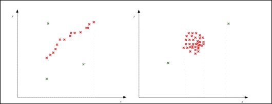
Some examples of outliers can be depicted by the following plots, where the red crosses mark normal observations and the green crosses mark the anomalous observations:

One possible approach to anomaly detection is to use a probability distribution model, which is built from the training data to detect anomalies. Techniques that use this approach are termed as statistical methods of anomaly detection. In this approach, an anomaly will have a low probability with respect to the overall probability distribution of the rest of the sample data. Hence, we try to fit a model onto the available sample data and use this formulated model to detect anomalies. The main problem with this approach is that it's hard to find a standard distribution model for stochastic data.

Another method that can be used to detect anomalies is a proximity-based approach. In this approach, we determine the proximity, or nearness, of a set of observed values with respect to the rest of the values in the sample data. For example, we could use the K-Nearest Neighbors (KNN) algorithm to determine the distances of a given observed value to its k nearest values. This technique is much simpler than estimating a statistical model over the sample data. This is because it's easier to determine a single measure, which is the proximity of an observed value, than it is to fit a standard model on the available training data. However, determining the proximity of a set of input values could be inefficient for larger datasets. For example, the KNN algorithm has a time complexity of , and computing the proximity of a given set of values to its k nearest values could be inefficient for a large value of k. Also, the KNN algorithm could be sensitive to the value of the neighbors k. If the value of k is too large, clusters of values with less than k individual sets of input values could be falsely classified as anomalies. On the other hand, if k is too small, some anomalies that have a few neighbors with a low proximity may not be detected.

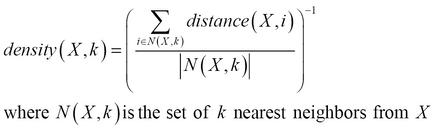
We can also determine whether a given set of observed values is an anomaly based on the density of data around it. This approach is termed as the density-based approach to anomaly detection. A given set of input values can be classified as an anomaly if the data around the given values is low. In anomaly detection, the density-based and proximity-based approaches are closely related. In fact, the density of data is generally defined in terms of the proximity or distance of a given set of values with respect to the rest of the data. For example, if we use the KNN algorithm to determine the proximity or distance of a given set of values to the rest of the data, we can define the density as the reciprocal of the average distance to the k nearest values, as follows:

Clustering-based approaches can also be used to detect anomalies. Essentially, clustering can be used to determine groups or clusters of values in the sample data. The items in a cluster can be assumed to be closely related, and anomalies are values that cannot be related to previously encountered values in the clusters in the sample data. Thus, we could determine all the clusters in the sample data and then mark the smallest clusters as anomalies. Alternatively, we can form clusters from the sample data and determine the clusters, if any, of a given set of previously unseen values.

If a set of input values does not belong to any cluster, it's definitely an anomalous observation. The advantage of clustering techniques is that they can be used in combination with other machine learning techniques that we previously discussed. On the other hand, the problem with this approach is that most clustering techniques are sensitive to the number of clusters that have been chosen. Also, algorithmic parameters of clustering techniques, such as the average number of items in a cluster and number of clusters, cannot be determined easily. For example, if we are modeling some unlabeled data using the KNN algorithm, the number of clusters K would have to be determined either by trial-and-error or by scrutinizing the sample data for obvious clusters. However, both these techniques are not guaranteed to perform well on unseen data.

In models where the sample values are all supposed to conform to some mean value with some allowable tolerance, the Gaussian or normal distribution is often used as the distribution model to train an anomaly detector. This model has two parameters—the mean and the variance . This distribution model is often used in statistical approaches to anomaly detection, where the input variables are normally found statistically close to some predetermined mean value.

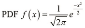
The Probability Density Function (PDF) is often used by density-based methods of anomaly detection. This function essentially describes the likelihood that an input variable will take on a given value. For a random variable x, we can formally define the PDF as follows:

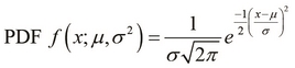
The PDF can also be used in combination with a normal distribution model for the purpose of anomaly detection. The PDF of a normal distribution is parameterized by the mean and variance of the distribution, and can be formally expressed as follows:

We will now demonstrate a simple implementation of an anomaly detector in Clojure, which is based on the PDF for a normal distribution as we previously discussed. For this example, we will use Clojure atoms to maintain all states in the model. Atoms are used to represent an atomic state in Clojure. By atomic, we mean that the underlying state changes completely or doesn't change at all—the changes in state are thus atomic.

We now define some functions to help us manipulate the features of the model. Essentially, we intend to represent these features and their values as a map. To manage the state of this map, we use an atom. Whenever the anomaly detector is fed a set of feature values, it must first check for any previous information on the features in the new set of values, and then it should start maintaining the state of any new features when it is necessary. As a function on its own cannot contain any external state in Clojure, we will use closures to bind state and functions together. In this implementation, almost all the functions return other functions, and the resulting anomaly detector will also be used just like a function. In summary, we will model the state of the anomaly detector using an atom, and then bind this atom to a function using a closure.

We start off by defining a function that initializes our model with some state. This state is essentially a map wrapped in an atom by using the atom function, as follows:

(defn update-totals [n]
  (comp #(update-in % [:count] inc)
        #(update-in % [:total] + n)
        #(update-in % [:sq-total] + (Math/pow n 2))))

(defn accumulator []
  (let [totals (atom {:total 0, :count 0, :sq-total 0})]
    (fn [n]
      (let [result (swap! totals (update-totals n))
            cnt (result :count)
            avg (/ (result :total) cnt)]
        {:average avg
         :variance (- (/ (result :sq-total) cnt)
                      (Math/pow avg 2))}))))

The accumulator function defined in the preceding code initializes an atom and returns a function that applies the update-totals function to a value n. The value n represents a value of an input variable in our model. The update-totals function also returns a function that takes a single argument, and then it updates the state in the atom by using the update-in function. The function returned by the accumulator function will use the update-totals function to update the state of the mean and variance of the model.

We now implement the following PDF function for normal distribution that can be used to monitor sudden changes in the feature values of the model:

(defn density [x average variance]
  (let [sigma (Math/sqrt variance)
        divisor (* sigma (Math/sqrt (* 2 Math/PI)))
        exponent (/ (Math/pow (- x average) 2)
                    (if (zero? variance) 1
                        (* 2 variance)))]
    (/ (Math/exp (- exponent))
       (if (zero? divisor) 1
           divisor))))

The density function defined in the preceding code is a direct translation of the PDF function for normal distribution. It uses functions and constants from the Math namespace such as, sqrt, exp, and PI to find the PDF of the model by using the accumulated mean and variance of the model. We will define the the density-detector function as shown in the following code:

 (defn density-detector []
  (let [acc (accumulator)]
    (fn [x]
      (let [state (acc x)]
        (density x (state :average) (state :variance))))))

The density-detector function defined in the preceding code initializes the state of our anomaly detector using the accumulator function, and it uses the density function on the state maintained by the accumulator to determine the PDF of the model.

Since we are dealing with maps wrapped in atoms, we can implement a couple of functions to perform this check by using the contains?, assoc-in, and swap! functions, as shown in the following code:

 (defn get-or-add-key [a key create-fn]
  (if (contains? @a key)
    (@a key)
    ((swap! a #(assoc-in % [key] (create-fn))) key)))

The get-or-add-key function defined in the preceding code looks up a given key in an atom containing a map by using the contains? function. Note the use of the @ operator to dereference an atom into its wrapped value. If the key is found in the map, we simply call the map as a function as (@a key). If the key is not found, we use the swap! and assoc-in functions to add a new key-value pair to the map in the atom. The value of this key-value pair is generated from the create-fn parameter that is passed to the get-or-add-key function.

Using the get-or-add-key and density-detector functions we have defined, we can implement the following functions that return functions while detecting anomalies in the sample data so as to create the effect of maintaining the state of the PDF distribution of the model within these functions themselves:

(defn atom-hash-map [create-fn]
  (let [a (atom {})]
    (fn [x]
      (get-or-add-key a x create-fn))))

(defn get-var-density [detector]
  (fn [kv]
    (let [[k v] kv]
      ((detector k) v))))

(defn detector []
  (let [detector (atom-hash-map density-detector)]
    (fn [x]
      (reduce * (map (get-var-density detector) x)))))

The atom-hash-map function defined in the preceding code uses the get-key function with an arbitrary initialization function create-fn to maintain the state of a map in an atom. The detector function uses the density-detector function that we previously defined to initialize the state of every new feature in the input values that are fed to it. Note that this function returns a function that will accept a map with key-value parameters as the features. We can inspect the behavior of the implemented anomaly detector in the REPL as shown in the following code and output:

user> (def d (detector))
#'user/d
user> (d {:x 10 :y 10 :z 10})
1.0
user> (d {:x 10 :y 10 :z 10})
1.0

As shown in the preceding code and output, we created a new instance of our anomaly detector by using the detector function. The detector function returns a function that accepts a map of key-value pairs of features. When we feed the map with {:x 10 :y 10 :z 10}, the anomaly detector returns a PDF of 1.0 since all samples in the data so far have the same feature values. The anomaly detector will always return this value as long as the number of features and the values of these features remains the same in all sample inputs fed to it.

When we feed the anomaly detector with a set of features with different values, the PDF is observed to change to a finite number, as shown in the following code and output:

user> (d {:x 11 :y 9 :z 15})
0.0060352535208831985
user> (d {:x 10 :y 10 :z 14})
0.07930301229115849

When the features show a large degree of variation, the detector has a sudden and large decrease in the PDF of its distribution model, as shown in the following code and output:

user> (d {:x 100 :y 10 :z 14})
1.9851385000301642E-4
user> (d {:x 101 :y 9 :z 12})
5.589934974999084E-4

In summary, anomalous sample values can be detected when the PDF of the normal distribution model returned by the anomaly detector described previously has a large difference from its previous values. We can extend this implementation to check some kind of threshold value so that the result is quantized. The system thus detects an anomaly only when this threshold value of the PDF is crossed. When dealing with real-world data, all we would have to do is somehow represent the feature values we are modeling as a map and determine the threshold value to use via trial-and-error method.

Anomaly detection can be used in both supervised and unsupervised machine learning environments. In supervised learning, the sample data will be labeled. Interestingly, we could also use binary classification, among other supervised learning techniques, to model this kind of data. We can choose between anomaly detection and classification to model labeled data by using the following guidelines: