By now we know the analysis work flow off by heart and as always the first step is getting to the required data. We have already detailed the steps involved in data extraction with Foursquare APIs. So instead of restating the obvious, we will start with the process of data extraction.

We have written two utility functions for the extraction of tips data from the identified end point:

Let's take an example of the extraction of tips data. We will find out the ID of the venue by browsing to the Foursquare page. This is the URL for the Vasa Museum in Stockholm:

https://foursquare.com/v/vasamuseet/4adcdaeff964a520135b21e3

The identified bold area in the URL is the ID that our function will need for data extraction:

# Extract data for Vasa Museum
vasa_museum_id = "4adcdaeff964a520135b21e3"
tips_df <- extract_all_tips_by_venue(vasa_museum_id)

The resultant DataFrame will look like this:

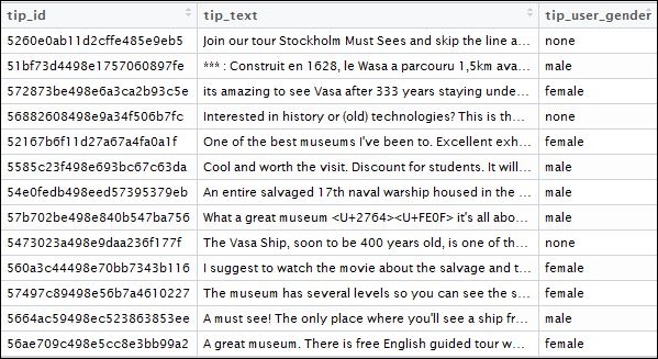
Tips for Vasa Museum, Stockholm

In addition to the tips, we have also extracted the gender of the tip user. This will help us with some interesting insights once we get started with our analytics step with the data.

This use case is an attempt to use the textual data and then use the sentiments arising out of that text to guide us in a decision-making process. For illustrating this concept, we have decided to pit the museum ratings from the popular travel site, TripAdvisor (https://www.tripadvisor.com) against the sentiment ratings from the users of Foursquare. We would like to find out if the sentiment of Foursquare users' tips are in agreement with the rankings given by TripAdvisor or not. This use case once again is a little bit speculative but it builds on the fundamentals of sentiment analysis we picked up in Chapter 2, Twitter – What's Happening with 140 Characters. The concepts and the idea behind sentiment analysis were explained in detail in Chapter 2, Twitter – What's Happening with 140 Characters, hence here we will get started with the use case directly. So let's see if the TripAdvisor ratings are validated by Foursquare users or not.

This is the list for the world's best museums according to TripAdvisor (https://www.tripadvisor.in/TravelersChoice-Museums-cTop-g1). We will manually compile this list in a DataFrame with the corresponding ranking.

This will be the final DataFrame for the museum rankings:

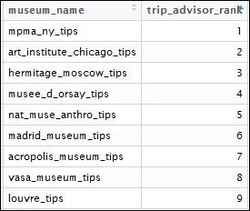
Museum rankings. Source https://www.tripadvisor.in/TravelersChoice-Museums-cTop-g1

The next step involves collecting the tips data for each of these museums. For this we will manually collect the Foursquare IDs for each of these museums and apply our tips extraction function on them. We have written a utility function which extracts data for each of these museums and then persists each of the DataFrame.

To perform analysis on the collective tips data, we will first start by concatenating the tips data for all the museums. We will assume that we have persisted data for each museum in a .csv file ending with _tips.

Using the following code, we will concatenate these files:

# Combine all the Tips data in a single data frame
tips_files <-list.files(pattern="*tips.csv")
complete_df <- data.frame()
for(file in tips_files)
{
    perpos <- which(strsplit(file, "")[[1]]==".")
    museum_name <- gsub(" ","",substr(file, 1, perpos-1))
    df <- read.csv(file, stringsAsFactors = FALSE)
    df$museum <- museum_name
    complete_df <- rbind(complete_df, df)
}

Now that we have all the data combined, we can get started with our analysis. Following up on the important caveat of the last section, we will start with some basic descriptive analysis.

Basic descriptive statistics

The first thing we want to see is how many tips there are for each of the museums. This is one of the initial requirements for the popularity of any venue.

Let us plot the number of total tips for each of these museums:

# Basic Descriptive statistics
review_summary <- complete_df %>% group_by(museum) %>% summarise(num_reviews = n())
ggplot(data = review_summary, aes(x = reorder(museum, num_reviews), y = num_reviews)) +
    geom_bar(aes(fill = museum), stat = "identity") +
    theme(legend.position = "none") +
    xlab("Museum Name") + ylab("Total Reviews Count") + ggtitle("Reviews for each Museum") +
    theme(axis.text.x=element_text(angle=90,hjust=1,vjust=0.5)) + coord_flip()

The accompanying graph reveals our first important finding. Although the Louvre, Paris is ranked quite low in the TripAdvisor ratings, the number of tips generated paints a different picture all together. It suggests that the Louvre should be the highest ranking museum. Another important difference is in the ranking of the National Museum of Anthropology, Mexico. Ranked 5th in the TripAdvisor, its popularity nose dives and it ends up at the bottom spot. These are some obvious outputs based on the number of tips, although we should not read much into it as we should be making such conclusions on the cumulative content of the tips and not just the number. Before we dig down to the level of sentiment of these tips, let us see if the rankings remain constant when we consider the gender of the user:

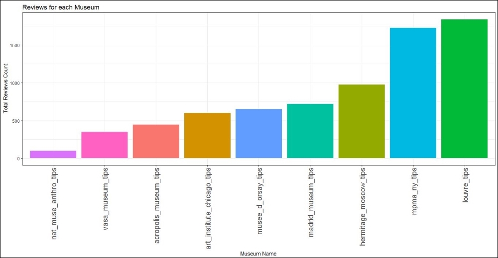
Museum rankings by tips

The plot for the three different genders (yes three because Foursquare also allows accounts having none as a gender), for the male and female gender the ranking is the same as the cumulative rankings. This tells us that gender is not a huge discriminant when it comes to leaving tips for a museum. Both genders are pretty consistent in their evaluation of the museums:

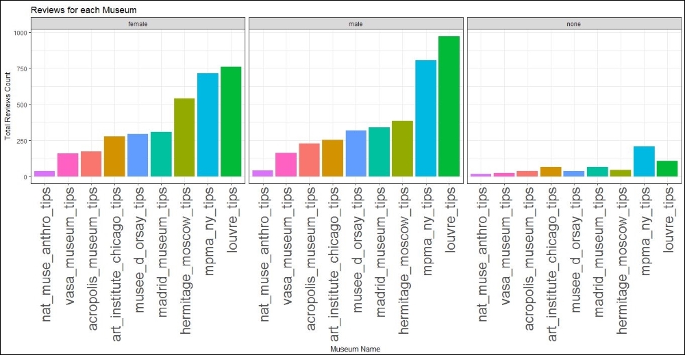
Museum rankings by tips for each gender

Next we want to examine the emotions that any visit to these museums generate. Are the emotions consistent across all the museums or can we identify different sentiments to attribute to different museums? To examine this, we will use the syuzhet package as we used in Chapter 2, Twitter – What's Happening with 140 Characters. We recall that given any text data, the syuzhet package helps us find the different sentiments reflected in that text. For the related information about the package and the working please refer to the excellent introduction provided in Chapter 2, Twitter – What's Happening with 140 Characters.

The following snippet will generate and plot a sentiment-based summary for each of our museums:

# Sentiments across different museums
sentiments_df <- get_nrc_sentiment(complete_df[,"tip_text"])
sentiments_df <- cbind(sentiments_df, complete_df[,c("tip_user_gender","museum")])
sentiments_summary_df <-sentiments_df %>% select(-c(positive,negative)) %>%
    group_by(museum) %>% summarise(anger = sum(anger),anticipation = sum(anticipation),disgust = sum(disgust), fear= sum(fear) , joy = sum(joy) , sadness = sum(sadness), surprise = sum(surprise), trust =sum(trust))
    
sentiments_summary_df_reshaped <- reshape(sentiments_summary_df,varying = c(colnames(sentiments_summary_df)[!colnames(sentiments_summary_df) %in% c("museum")]), v.names = "count", direction = "long",new.row.names = 1:1000)
sentiment_names <-c(colnames(sentiments_summary_df)[!colnames(sentiments_summary_df) %in% c("museum")])
sentiments_summary_df_reshaped$sentiment <- sentiment_names[sentiments_summary_df_reshaped$time]
sentiments_summary_df_reshaped[,c("time", "id")] <- NULL

p5 <- ggplot(sentiments_summary_df_reshaped, aes(x=sentiment, y=count))
(p5 <- p5 + geom_bar(stat="identity") + theme(axis.text.x=element_text(angle=90,hjust=1,vjust=0.5)) +
        facet_wrap(~museum, ncol = 1)) +
        ylab("Percent sentiment score") + 
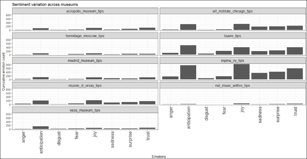
        ggtitle("Sentiment variation across museums")

The output of the preceding code snippet will give us a distribution of all the sentiments across the different museums. The plot is given here:

Sentiment score for each museum

A careful reading of the preceding plot reveals some important information about the sentiments dominating the tips for them. Anticipation, joy, and trust are the major sentiments across all the museum visitors, which is exactly what one would expect. It is nice to find corroborating data for our human intuitions. It also reveals something about the museums in New York and Paris: they often experience a sentiment of disgust and anger by the users visiting them, which is not something which you would expect when visiting the world's top most museums.

This sentiment analysis helps us get some insights into the museums and the sentiments associated with them but we can't use them directly to achieve our initial goal: building a sentiment-based ranking of the museums. To build that, we need a numerical definition of sentiment. Thankfully, the package which we are using has functions to do precisely that. To arrive at our rankings, we will associate a sentiment score with each of the textual tips and sum them to arrive at a cumulative total. Sounds nice but this approach has a flaw in it; we need to take into account the number of tips also. Otherwise, the museums with a large number of tips will be favored. To counter such fallacies, we will do a tip count-based normalization. This will remove the effect of the large number of tips for each of the museums. We will be left with a metric of per tip sentiment score which we can use to rank the museums:

# Sentiment analysis based ranking
#Ranking based on cumulative review sentiments
for (i in 1:nrow(complete_df)){
    review <- complete_df[i,"tip_text"]
    poa_word_v <- get_tokens(review, pattern = "\W")
    syuzhet_vector <- get_sentiment(poa_word_v, method="bing")
    complete_df[i,"sentiment_total"] <- sum(syuzhet_vector)
}
rank_sentiment_score <- complete_df %>% group_by(museum)%>% summarise(total_sentiment = sum(sentiment_total), total_reviews = n()) %>% mutate(mean_sentiment = total_sentiment/total_reviews) %>% arrange(mean_sentiment)
rank_sentiment_score$museum.rank <- rank(-rank_sentiment_score$mean_sentiment)

rank_sentiment_score_gender <- complete_df %>% group_by(museum, tip_user_gender)%>% summarise(total_sentiment = sum(sentiment_total), total_reviews = n()) %>% mutate(mean_sentiment = total_sentiment/total_reviews) %>% arrange(mean_sentiment)

rank_sentiment_score_gender_female <- subset(rank_sentiment_score_gender, tip_user_gender == "female")
rank_sentiment_score_gender_female$museum.rank <- rank(-rank_sentiment_score_gender_female$mean_sentiment)

rank_sentiment_score_gender_male <- subset(rank_sentiment_score_gender, tip_user_gender == "male")
rank_sentiment_score_gender_male$museum.rank <- rank(-rank_sentiment_score_gender_male$mean_sentiment)

rank_sentiment_score_gender_none <- subset(rank_sentiment_score_gender, tip_user_gender == "none")
rank_sentiment_score_gender_none$museum.rank <- rank(-rank_sentiment_score_gender_none$mean_sentiment)

# All the ranks in one data frame
combined_rank <- museum_tripadvisor %>% inner_join(rank_sentiment_score[,c("museum", "museum.rank")])
colnames(combined_rank)[ncol(combined_rank)] <- "overall_sentiment_rank"
combined_rank<- combined_rank %>% inner_join(rank_sentiment_score_gender_female[,c("museum", "museum.rank")], by = "museum")
colnames(combined_rank)[ncol(combined_rank)] <- "female_sentiment_rank"
combined_rank<- combined_rank %>% inner_join(rank_sentiment_score_gender_male[,c("museum", "museum.rank")], by = "museum")
colnames(combined_rank)[ncol(combined_rank)] <- "male_sentiment_rank"
combined_rank<- combined_rank %>% inner_join(rank_sentiment_score_gender_none[,c("museum", "museum.rank")], by = "museum")
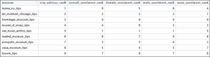
colnames(combined_rank)[ncol(combined_rank)] <- "none_sentiment_rank"

This summarization helps us arrive at our new set of rankings based on the metric of mean sentiment score per user. So basically we are saying that based on the cumulative sentiments of tips generated for each of the museums, we can find out which museum can be ranked higher. We can contrast this with the ranks given by TripAdvisor to find out whether these ranks are in agreement or not. Furthermore, we are able to rank the museums based on the same metric for each gender.

Let's see how the results of this summarization look:

Sentiment score for each museum

This will formally conclude our text-based analysis on the tips data. We learned a fair deal about extracting sentiments from textual data and also how to use the numerical values of sentiments to perform important analytics.