The first step in any data-mining task is to perform some data-cleaning tasks. The specific methods selected for cleaning will often depend on the nature of the data. We will perform a few very basic steps to achieve the required sanity of our data. The following code will perform the basic cleaning tasks for us. The code is commented to give the function that we are performing. We have already explained the logic of these functions in Chapter 2, Twitter – What's Happening with 140 Characters, and the user can refer to it for more details:

articles_phase1 <- articles_df %>% filter(time_interval == "Phase 1")
articles_phase1 <- Corpus(VectorSource(articles_phase1[,"content"]))

# Convert all text to lower case
articles_phase1 <-tm_map(articles_phase1,content_transformer(tolower))

# Remove all punctuations from the text
articles_phase1 <- tm_map(articles_phase1, removePunctuation)

# Remove all numbers from the text
articles_phase1 <- tm_map(articles_phase1, removeNumbers)

# Remove all english stopwords from the text
articles_phase1 <- tm_map(articles_phase1, removeWords, stopwords("english"))

# Remove all whitespaces from the text
articles_phase1 <- tm_map(articles_phase1, stripWhitespace)

The most important decision to be taken at this stage is the representation of the documents we want to use. This numerical representation is used by text-mining algorithms. The simplest representation is the bag-of-words representation. In this representation, we find out the total words in the corpus, and each document is represented as the numerical vector of its constituent words.

Here is a very simple example of a term matrix. Suppose we have two documents in the corpus, as given here:

Before we convert our text data into such a representation, we will also stem the data; that is, we will reduce all the words to their base forms. Once we have completed these two steps, we will have a representation of our document, which we can then use for topic modeling. The following code will perform these two actions:

# Stem all word in the text
articles_phase1 <- tm_map(articles_phase1,stemDocument)

# Creating a Document term Matrix
dtm_trump_phase2 <- DocumentTermMatrix(articles_phase1)

Please note that we will not include the code for cleaning and processing the second phase of articles. The reader can easily do this themself using the preceding sequence of code.

Once we are done with both of these two tasks, we can proceed with our topic modeling task. We will be using the topicmodels package to fit one of the most famous topic models, LDA, using an algorithm called Gibbs sampling. The process of fitting a topic model onto our dataset is quite straightforward. It can simply be achieved by calling the LDA function of the package. The following code will generate the topic models for both phases of our data. First, we will analyze the results that we get out of our initial models and then we will discuss what the tuning process may look like if the reader is looking for a more involved reiteration of the process:

burnin <- 4000
iter <- 200
thin <- 500
seed <-list(2003,5,63,100001,765)
nstart <- 5
best <- TRUE

#Number of topics
k <- 5

#Run LDA using Gibbs sampling
ldaOut <-LDA(dtm_trump_phase1,k, method="Gibbs", 
             control=list(nstart=nstart, seed = seed, best=best, burnin = burnin, iter = iter))

To develop our model, we set some parameters (mostly defaults from the vignette of the package) and then call the LDA function with the method set as "Gibbs". This selects the particular model-fitting procedure from the set of algorithms that can be used to perform the task. Another important parameter, and also a limitation of LDA, is the number of topics value. It is unlikely that you will be able to know how many types of topics there are in the corpus, so this value is often selected by the practitioners on the basis of domain-knowledge-based intuition. Once we get the initial results, we can go ahead and try different values of this parameter to get better topics.

The output of the preceding function will include the probability of each topic for every document in the corpus and the terms associated with each of the topics, among other things. Now comes the tricky part, which makes topic modeling useful but slightly tough to use. Before we come to that, let's see what the top 10 terms associated with each of the topics are for both our phases. The following code will generate those terms:

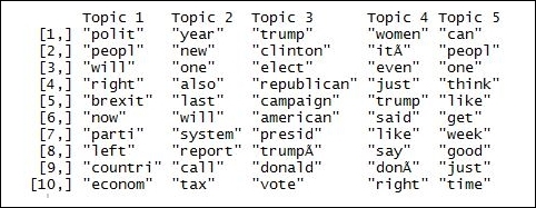
ldaOut.terms <- as.matrix(terms(ldaOut,10))
ldaOut.terms

The output of the code is given in the following image:

Topics in phase 1

The output will not give us very identifiable topics by itself. It will help us with the terms that can be associated with the topics, and then the user can make a call and label the topic accordingly. For example, it is tough to label Topic 1 here, but we can see common themes in the other topics. Topic 5 probably deals with Mr. Trump's major promotion theme. Topic 2 can be termed Mr. Trump's comparison to the opponent. Topic 3 is again tough to classify, but Topic 4 can be attributed to Mr. Trump's appeal to the voters. This is a very subjective task and hence, although the procedure is very powerful, it is far from a magic wand.

Let us complete this discussion by taking a look at the topics from phase 2. The following image gives the similar terms output for the second phase of articles:

Topics in phase 2

The topics in the second phase seem a little more defined. We still have some similar topics to the first phase but the biggest difference is the terms for Topic 1. We clearly see that this topic deals with some policy-related questions. Also gone is the topic from phase 1 that dealt with some controversial topics (refer to Topic 5 in the earlier image). The story it paints is an interesting one. Post the confirmation of his candidacy, the opinion writers shifted to focus on the policies of Mr. Trump, whereas earlier the focus was not so much on those issues. This capability of topic modeling is what makes it a powerful tool for analyzing a large corpus of textual data.

The results of our primitive experiments are quite interesting. The reader can go back and tinker with the process to arrive at better/different results. There are broadly two ways in which we can achieve a little more refinement of the results:

As with our other modeling-related tasks, we will not go into the detailed process, but will give the reader a gentle introduction that can serve as a starting point for the future endeavors of the users.