For any clustering algorithm, the cohesiveness of clusters is an indicator of quality, that is, the closer the data points within a cluster are to its centroid the better it is. To quantify the same, we use a metric called Within the cluster distance to centroid or withiness or WCSS for short. We use this metric as a function of k (the k in k-means) to help us find the optimal value of it for the given dataset. Notice that, as the value of k increases, the value of WCSS decreases and approaches a minima.

In other words, we look at the variance explained by the clusters as a function of k. If we plot WCSS versus K, this variance sees an inflection; that is, there comes a point when any more clusters do not help in providing significant gains in terms of cluster quality. Hence, this point of inflection is what points towards optimal k.

It should be noted that the Elbow criteria gives us a ball-park value of k that may or may not be optimal. Yet it is a good enough criterion to narrow down the search for optimal k. The following sample plot shows how WCSS changes with the value of k and it also clearly shows the elbow or point of inflection at 5:

Elbow method for k-means

The Elbow method helps us narrow down the search space for k and, more often than not, provides us with a meaningful value as well. To further improve and use the correct value of k, there is another method called the Silhouette method.

The Elbow method works with WCSS as a function of k but does not take into account other factors. With the Silhouette method, we work with dissimilarities.

A Silhouette is defined as a measure of how close a data point is to its cluster and how far off it is from other clusters. Thus, the Silhouette method checks for both cohesiveness and separation between clusters. A value of 1 signifies a nice match while -1 points towards an incorrect cluster for a given data point.

To put it formally:

Here:

The average of s(i) for all data points in a cluster is a measure of how tightly its data points are grouped. The following is a sample silhouette plot. In the plot, each of the colored silhouettes represents a cluster with their average s(i) value and overall average silhouette value mentioned at the bottom of the plot. As we can see from the plot, some clusters are wider than others along with a difference in the number of members in each.

Silhouette plot for k-means

Now that we have details on how to find k for our k-means algorithm, let us apply this knowledge to our use case. The kmeans() function from the stats package provides an easy to use function. This function takes the DataFrame and number of clusters as input to generate a fit for our dataset.

Since we do not know the optimal value of k, let us employ the Elbow criterion to find it. The following snippet uses kmeans() in a loop with k varying from 1 to 15 clusters and collecting the withiness or WCSS value for each value of k in a vector withiness_vector:

# elbow analysis for kmeans
withiness_vector <- 0.0
for (i in 1:15){
  withiness_vector[i] <- sum(kmeans(nomissing_interesting,
                                     centers=i)$withinss)/(10^10)
}
# prepare dataframe for plotting
eblowDF <-data.frame(withiness_vector,1:15)
colnames(eblowDF)<-c("withiness",
                     "cluster_num")

Now that we have WCSS for different values of k, let us find our elbow point. The following snippet uses ggplot to generate the required plot:

# plot clusters with regions marked out
ggplot(data = eblowDF, 
       aes(x = cluster_num, 
           y = withiness)) +
geom_point() +
geom_line() +
labs(x = "number of clusters", 
     y = "scaled withiness",
     title="Elbow Analysis") +
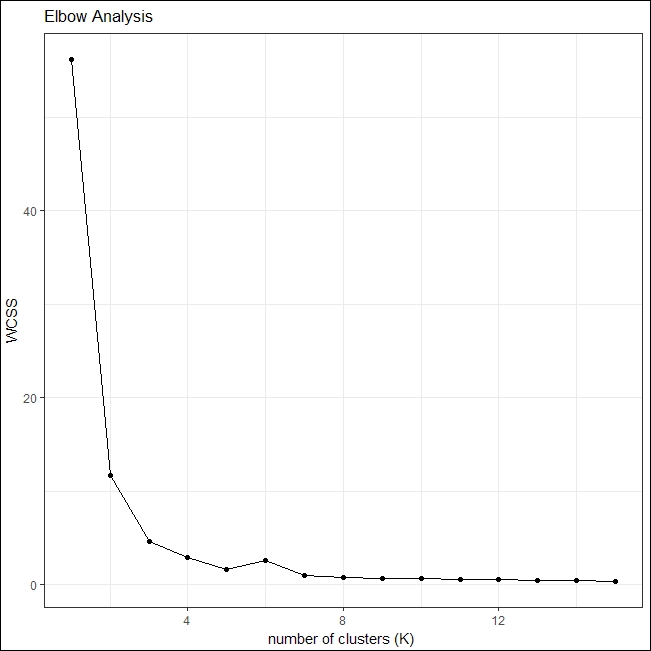
theme_ipsum_rc()

The generated plot points towards an optimal value of k as 4, after which the value of WCSS remains fairly constant:

Elbow plot for interesting photos

To validate our findings related to value of k, we apply the silhouette method for values of k, such as 3, 4, 5 and 6.

The following snippet uses the daisy() method from the cluster package to generate a dissimilarity matrix which we then use to plot and analyze the quality of clusters at k=4:

# silhouette analysis for kmeans
dissimilarity_matrix <- daisy(nomissing_interesting) 
plot(silhouette(fit$cluster, 
                dissimilarity_matrix), 
     col=1:length(unique(fit$cluster)), 
     border=NA)

The silhouette plot shows an average of 0.65 for k=4, which is maximum as compared to values observed at k=5 or 6.

The following is the plot in consideration. The plot also outlines similar Silhouette widths as well:

Silhouette plot for k=4

Once we have identified the value of k to work with, we regenerate the clustering output for our dataset on the interestingDF DataFrame.

The logical next step is to visualize how the clusters look. Using the output of our clustering step, we assign each data point its corresponding cluster number using the attribute $cluster from the fit object. Since the focal lengths are very thinly spread across our DataFrame, we aggregate the results, using ddply(), by taking the max of focal length as an indicator for each cluster. We also add a derived attribute called fl_bin. This attribute is a categorical value which describes focal length in one of seven bins we have decided upon. The following snippet gets us the required summary object:

# aggregate results
cluster_summary <- ddply(
                  nomissing_interesting,
                  .(iso, views,cluster_num),
                  summarize,
                  focal_length=max(focal_length)
                  )


# bin focal_lengths for plotting
cluster_summary$fl_bin <- sapply(cluster_summary$focal_length,binFocalLengths)
cluster_summary$fl_bin<- as.factor(cluster_summary$fl_bin)

The final step in this puzzle is to plot the clustered data points. For this we again rely on ggplot as usual. The following snippet generates the required plot with each of the cluster regions clearly marked out. To visualize all three dimensions (iso, views and focal length): the plot uses colors to identify clusters, x and y axis to denote views and iso respectively, and shapes to mark focal length bins:

# plot clusters with regions marked out
ggplot(data = cluster_summary, 
       aes(x = views, 
           y = iso ,
           color=factor(cluster_num))) +
  geom_point(aes(shape=fl_bin)) + 
  scale_shape_manual(values=1:nlevels(cluster_summary$fl_bin)) +
  geom_polygon(data = hulls[hulls$cluster_num==1,], 
               alpha = 0.1,show.legend = FALSE) + 
  geom_polygon(data = hulls[hulls$cluster_num==2,], 
               alpha = 0.1,show.legend = FALSE) +
  geom_polygon(data = hulls[hulls$cluster_num==3,], 
               alpha = 0.1,show.legend = FALSE) +
  geom_polygon(data = hulls[hulls$cluster_num==4,], 
               alpha = 0.1,show.legend = FALSE) +
  labs(x = "views", y = "iso",title="Clustered Images") +
  theme_ipsum_rc()

The following is the generated plot:

Metering mode wise photo distribution

As we can see with the preceding plot, the clusters are nicely defined across the attributes of our dataset. Focal lengths are more or less distributed across clusters, with each cluster visually being limited by view count. Also, it is interesting to see that clusters 2, 3 and 4 all have images clicked with a lens of focal length between 10-20mm have maximum iso values.

Further investigation of individual clusters may help uncover further insights. We'll leave this as an exercise for the readers to explore.