Exchangeable Image File Format (EXIF) is a format used by digital cameras, smartphones, and other devices to handle and store information related to images, sounds, videos, and so on. It is a long-standing standard, first released in the mid-1990s, and now widely used by digital devices with photographic capabilities. Without going into too much detail, EXIF defines how and what all metadata related to images, sounds and videos is stored by these devices and/or editing software such as Adobe Photoshop, Gimp and the likes.

Some of the most commonly found metadata attributes in image files are:

EXIF metadata or EXIF for short is not just used for the handling of digital images by software and hardware but is used in common lingo by professional photographers as well. Photographers use EXIF to discuss and convey details about how a particular image was taken, using what camera and lens, in a concise and standard format, which is consistent across images taken using cameras from different manufacturers.

The following is a snapshot showcasing a particular image's EXIF information:

EXIF Sample [source: By Sysy~commonswiki - Own work, Public Domain, https://commons.wikimedia.org/w/index.php?curid=1468710]

Getting a bit of a background about the domain certainly helps. Now that we have a brief understanding of EXIF, let us proceed and extract EXIF information for the interesting photos we have extracted.

Similar to interestingness, Flickr has a separate API endpoint to extract EXIF information. To get to the EXIF information, this API endpoint requires an image's corresponding photo.id and photo.secret which is available to us in our base DataFrame. We write another small utility function to use this API endpoint as follows:

# utility function to get EXIF for an image.
getEXIF<- function(image){
exif <- GET(url=sprintf(
"https://api.flickr.com/services/rest/?method=flickr.photos.getExif&api_key=%s&photo_id=%s&secret=%s&format=json&nojsoncallback=1"
              , api_key
      , interestingDF[image,"id"]
      , interestingDF[image,"secret"]
        )
      ) %>>%
      content( as = "text" ) %>>%
      jsonlite::fromJSON ()
}

Using the preceding utility function, we simply iterate over our base DataFrame interestingDF to get each image's EXIF data.

The following snippet performs the previously mentioned action:

# get exif information for each image
exifData <- lapply(1:nrow(interestingDF),
                   getEXIF)

We now proceed towards extracting and preprocessing individual EXIF attributes from exifData object. As we saw previously with interestingness data, the EXIF response object is also a complex nested structure. We make use of pipeR, plyr and dplyr to get to relevant attributes. The following code snippet extracts ISO and camera make information from exifData object:

# Use EXIF Data to get specific attributes
# ISO
iso_list <- as.numeric(exifData %>>%
                         list.map(as.numeric(
                           as.data.frame(.$photo$exif)[
                             which(.$photo$exif["label"]=="ISO,
                              Speed"),"raw"])
)
)

# Manufacturer/Make
make_list <- exifData %>>% 
                  list.map(unlist(
                    as.data.frame(
                      .$photo$exif)[
                        which(.$photo$exif["label"]=="Make"),
                        "raw"] )[1] %>>% as.character
                  )%>>% as.character

# handle missing make information
make_list <- ifelse(make_list=="character(0)",
                    NA,
                    make_list)

In a similar manner, we extract details related to focal length, white balance, metering mode, and so on with pre/post processing as required for the particular attribute.

We now merge these individual attributes of EXIF metadata to our main DataFrame as follows:

# Add attributes to main data frame
interestingDF$iso <- iso_list
interestingDF$make <- make_list
interestingDF$focal_length <- focal_list
interestingDF$white_balance <- whiteBalance_list
interestingDF$metering_mode <- meteringMode_list

The additional attributes of the updated DataFrame are shown in the following snapshot. It has all the additional EXIF attributes we extracted in the preceding steps:

InterestingnessDF with EXIF attributes

Flickr also provides view counts for each of the images available on the platform. To get to the view count information, we write another utility function using the getInfo API end point. This endpoint returns tags and view counts on a per image basis. We use the following snippet to extract view counts for images in our base DataFrame:

# get tag and view count data
tagData <- lapply(1:nrow(interestingDF),
                  getInfo)

# Image View Count
views_list <- as.numeric(tagData %>>% 
                           list.map(
                             unlist(.$photo$views)) %>>% 
                           as.character)

We merge this additional attribute as well with our main DataFrame interestingDF.

Now that we have our base DataFrame enhanced with additional information in the form of EXIF attributes and view counts, we should wear our data science hats and get started with some initial exploratory analysis of this dataset.

The following is a quick summary of the DataFrame using the function summary() to begin with:

Summary of InterestingnessDF

The summary of the DataFrame gives us a nice overview of the quality of the data. Apart from information related to min/max and other statistical attributes, we get to know that about 65-70% of the data is populated across all available attributes. We may have to work out a strategy to handle this missing information by using our domain knowledge and other methods learned in previous chapters. We may also choose to ignore rows with missing information if we can work with a reduced dataset.

Let us make use of ggplot to visualize some of these attributes to get a better understanding of the data. The following snippet plots the frequency distribution of images based on different makes/manufacturers:

# Plot images counts by make
ggplot(interestingDF[!is.na(interestingDF$make),], 
       aes(make)) +
  geom_bar() + 
  coord_flip() +
  labs(x="Make", y="Image Counts",
       title="Make wise Image distribution"
        ) + 
  theme_ipsum_rc(grid="XY")

The output plot is as follows:

Make wise photo distribution

The preceding plot clearly shows that the most interesting photos are being clicked using Canon and Nikon cameras. These two are followed by other DSLR manufacturers, with a minor presence from smartphones such as the Apple iPhone.

This plot also points towards two interesting insights. Firstly, it seems that Flickr's set of interesting images for this brief 10-day period seems to have a lot more DSLR clicked images as compared to other image sharing websites/platforms like Instagram, which primarily cater to the smartphone audience. Secondly, it points us towards a potential data issue which would require some further preprocessing to achieve better results. If we look closely, there are a few manufacturers, such as Nikon, Olympus, and others, that have multiple entries in the plot due to different names available as part of the EXIF data. This may be due to different models, post-processing software, or other reasons.

Along the same lines, let's see how the distribution related to the metering mode is spread. We again make use of our friendly ggplot() as shown in the following snippet:

ggplot(interestingDF[!is.na(interestingDF$metering_mode),], 
       aes(metering_mode)) +
  geom_bar()+ 
  coord_flip() +
  labs(x="Metering Mode", y="Image Counts",
       title="Metering Mode wise Image distribution"
  ) + 
  theme_ipsum_rc(grid="XY")

The metering mode distribution is as follows:

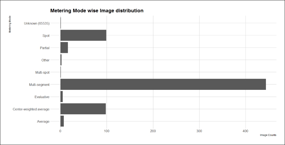
Metering mode-wise photo distribution

Multi-segment seems to be the favorite here, followed by spot and center-weighted average metering modes. The high counts for spot and center-weighted average may point towards quite a sizeable number of images being portraits, or to images with subjects in the middle. Further analysis would require a deeper understanding of these metering modes which is beyond the scope of this chapter.