Before we get started with building a classifier to answer the preceding question, we need some more data. Apart from the data we have collected so far (corresponding to interesting images only), we need to collect data related to photos which have never made it to the Explore page. Employing techniques similar to those we have used for collecting data for interesting photos, we'll use the getpublicphotos API to get the other set of photos.

The following snippet uses that API to build a utility function called getPhotosFromFlickr based on the user_id provided:

# extract photos of given user_id
# use flickr.people.getpublicphotos
getPhotosFromFlickr <- function(api_key,
                                token,
                                user_id){
  GET(url=sprintf(
 "https://api.flickr.com/services/rest/?method=flickr.people.getpublicphotos&api_key=%s&user_id=%s&format=json&nojsoncallback=1"
    , api_key
    , user_id
    , token$credentials$oauth_token
  )
  ) %>>%
    content( as = "text" ) %>>%
    jsonlite::fromJSON () %>>%
    ( .$photos$photo ) %>>%
    ( data.frame(
      .
      ,stringsAsFactors=F
    ))
}

We reuse the utilities for extracting EXIF and view counts for each of the images we extract for user_ids. The following snippet shows the utility function which returns a DataFrame of photos for a given user_id using the utilities developed so far:

# Get Photos for given user_id
getUserPhotos <- function(api_key,
                          token,
                          user_id){
  
  #get user's photos in a dataframe
  photosDF <- getPhotosFromFlickr(api_key,token,user_id)
  
  # get exif for each photo in dataframe
  photos.exifData <- getEXIF(api_key,photosDF)
  

  # Image ISO
  iso_list <- extractISO(photos.exifData)
  
  # Image Manufacturer/Make
  make_list <- extractMakes(photos.exifData)                         
  
  # Image Focal Length
  focal_list <- extractFocalLength(photos.exifData)
  
  # Image White Balance
  whiteBalance_list<-extractWB(photos.exifData)
  
  # Image Metering Mode
  meteringMode_list <- extractMeteringMode(photos.exifData)
  
  
  # Add attributes to main data frame
  photosDF$iso <- iso_list
  photosDF$make <- make_list
  photosDF$focal_length <- focal_list
  photosDF$white_balance <- whiteBalance_list
  photosDF$metering_mode <- meteringMode_list
  
  # get view counts
  photosDF$views <-   getViewCounts(api_key,photosDF) 
  
  as.data.frame(photosDF)
}

The output DataFrame consists of all the attributes we have in the interestingDF DataFrame with the attributes correctly type-casted.

Most classification algorithms expect the features to be numeric in nature. In our dataset, attributes such as iso, focal_length, and views are already numeric. Since the make of the camera used to take the photo, along with settings like white balance and metering mode, have a significant impact on the outcome, we'll convert these attributes to factors.

The following snippet typecasts the attributes to be used by the classification algorithm:

# typecast dataframes for use by classifier
prepareClassifierDF <- function(classifyDF){
  
  # convert white balance to factor and then encode numeric
  classifyDF$white_balance <- as.factor(classifyDF$white_balance)
  
  # convert metering mode to factor
  classifyDF$metering_mode <- as.factor(classifyDF$metering_mode)
  
  # convert make_clean to factor
  classifyDF$make_clean <- as.factor(classifyDF$make_clean)
  
  as.data.frame(classifyDF)
}

We use the utility getUserPhotos to extract photos from a randomly chosen set of Flickr accounts and prepare a DataFrame consisting of negative examples, that is, photos which have never made it to the Explore page. The following snippet iterates through a list of user_ids listed in the list mortal_userIDs and assigns a classification label of 0 to each entry. We similarly assign a class label 1 to all our photos in the DataFrame interestingDF:

neg_interesting_df <- lapply(mortal_userIDS,
                          getUserPhotos,
                          api_key=api_key,token=tok) %>>%
                      ( do.call(rbind, .) )


neg_interesting_df <- na.omit(neg_interesting_df)
neg_interesting_df$is_interesting <- 0

# Photos from Explore page
pos_interesting_df <- na.omit(interesting)
pos_interesting_df$is_interesting <- 1

We use rbind() to concatenate both positive and negative examples in a common DataFrame and then restrict the set of attributes to only iso, focal_length, views, white_balance, metering_mode, and make_clean. The following snippet performs these actions:

# prepare overall dataset
classifyDF <- rbind(pos_interesting_df[,colnames(neg_interesting_df)],
                    neg_interesting_df)

# restrict columns 
req_cols <- c('is_interesting',
             'iso',
             'focal_length',
             'white_balance',
             'metering_mode',
             'views',
             'make_clean')

classifyDF <- classifyDF[,req_cols]

Now that we have our dataset ready, we have one last step before we learn from the data to build a classifier: we need to split our data in training and testing samples. Without going into much detail, a supervised learning algorithm is provided with a set of data points with actual class labels to learn from. This dataset is called the training dataset. The algorithm is then tested for performance using another set of data points whose labels are not known to the algorithm. This is called the test dataset. Usually, there is another dataset called the validation dataset which is used to fine tune the algorithm and check for issues such as overfitting and so on.

The following snippet samples the classifyDF DataFrame into train and test datasets in 60:40 ratio:

# train - test split
set.seed(42)
samp <- sample(nrow(classifyDF), 0.6 * nrow(classifyDF))
train <- classifyDF[samp, ]
test <- classifyDF[-samp, ]

Now that we have our features in the required shape and the data split into training and testing sets, we can proceed towards building our classifier. For the current use case, we will build a classifier based on the random forest classification algorithm, which is available from the caret package. We'll pass the train DataFrame with formula denoting is_interesting as the class label based on all other attributes to train(). This function also takes input to preprocess the data, and we use scaling since our attributes are measures of different qualities of a photo. We'll use the attribute trControl to cross validate our training model and improve performance against overfitting. The following snippet helps us learn a random forest classifier.

# train model
rfModel <- train(is_interesting ~ ., train,
                      preProcess = c("scale"),
                      tuneLength = 8,
                      trControl = trainControl(method = "cv"))

Now that we have our classifier ready, let's test its performance by generating some class predictions. For this we use our test dataset. The predict function takes the classifier model as input followed by the test dataset without the class labels. We use type= "prob" to generate output probabilities for each class label. Remember class label 0 refers to photos not making to the Explore page, while class label 1 refers to photos which have been listed on the Explore page. The following snippet generates the required predictions:

# Prediction
predictedProb <- predict(rfModel, test[,-1], type="prob")

To test the performance of our classifier, we use the Receiver Operating Characteristic (ROC) measure. ROC is available from the pROC package. The following snippet plots the ROC curve for our classifier:

# Draw ROC curve.
resultROC <- roc(test$is_interesting, predictedProb$"1")
plot(resultROC, 
     print.thres="best", 
     print.thres.best.method="closest.topleft")

#to get threshold and accuracy
resultCoords <- coords(resultROC, 
                        "best", 
                        best.method="closest.topleft", 
                        ret=c("threshold", "accuracy"))

The generated plot is shown in the following diagram. It clearly points towards a very nicely learned classifier, with an ROC curve lying well above the random guess and the highest accuracy of 98% approx at a threshold value of 0.68:

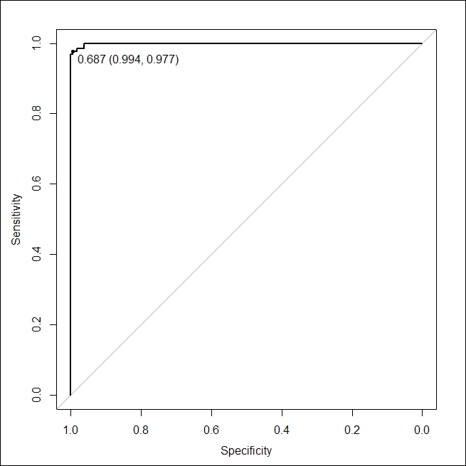
ROC curve for random forest classifier

The confusion matrix based on the test data also shows the classifier working correctly in the majority of the cases. The following is a snapshot of the confusion matrix:

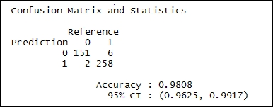
Confusion matrix for random forest classifier

Now that we have a classifier which has learned to classify between interesting and non-interesting images, let us put this classifier to the test. We use this random forest based classifier to classify images for another random set of user(s). You may try to test the classifier on your own images as well. For our current use case, we extracted public photos from one of our own accounts and then allowed the classifier to work and suggest labels. Note that we use the same predict function with type="prob". The following is the output generated by our classifier:

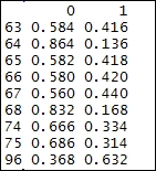
Class output probabilities by random forest classifier

In the preceding snapshot, the first column is the image identifier, while column 0 denotes probabilities for a photo not making it to the Explore page, and column 1 points to the probability of making it to the Explore page. Please note that each row's probabilities add up to 1 (as they should).

Since the images used for this test were from one of our own Flickr accounts, we already know that none of these photos have ever made it to the Explore page. Interestingly, the classifier works correctly for eight out of the nine photos while generating a wrong result for the last one!

Of course, far more sophisticated methods can also be employed, such as deep learning, convolutional neural networks, and so on, to improve the results. However, the results achieved in this section are still impressive and point towards the fact that we can answer questions related to them with a certain level of confidence. These topics are beyond the scope of this chapter but you are encouraged to learn more about them.