
7
Applying Machine Learning to Genomics
The genome is what defines a living organism. It resides in the cells of the organism and dictates how they perform essential functions. It is also what differentiates one organism from another by providing each organism a set of unique characteristics. Genomes form the complete deoxyribonucleic acid (DNA) of an organism. It resides mostly in the nucleus (and in small quantities within the mitochondria) of the cell and provides coded information about the organism by representing it in a sequence of four chemical bases: thymine (T), cytosine (C), guanine (G), and adenine (A). These are arranged in a double helix structure, which is now synonymous with how DNA is represented graphically. The double helix is comprised of two strands of nucleotides that bond with each other forming pairs of chemical bases (also known as base pairs), with A pairing with T and G pairing with C. Genomes may also contain sequences of ribonucleic acid (RNA), which is quite common in smaller organisms such as viruses. RNA contains shorter chains of nucleotides than DNA and is synthesized using the information stored in DNA in a process called transcription. This results in the formation of proteins and ultimately phenotypes, the characteristics of an organism that you can observe.
The human DNA molecule is arranged in structures called chromosomes within the cell nucleus. There are 23 pairs of chromosomes (X, Y) in a typical human cell forming a total of 46 chromosomes. The 23rd chromosome differs in males and females, with females having two X chromosomes and males having X and Y each. The human genome consists of about 3 billion base pairs of sequences of nucleic acids encoded in the human DNA, which resides in the nucleus of the cell. The Human Genome Project (HGP) was a scientific research project kicked off in 1990 and attempted to decode the sequence of the whole human genome, in a process called genetic sequencing. It covered 92% of the full human genome sequence as of 2003. Improvements in genomic sequencing technology and lab infrastructure over the years have led to massive gains in our understanding of the human genome. In April 2022, the final remaining 8% of the sequences of the human genome were identified and released. It’s fascinating to note that, generally speaking, while no two humans (except identical twins) look the same, it is only 0.1% of human genes that vary between individuals. This is testament to the fact that humans (or homo sapiens) are still a very young species compared to other life forms on Earth that pre-date humans by many centuries and, hence, have evolved with many more genetic variations. The 0.1% of genetic variation in humans is the basis of genomic research that attempts to identify how an individual is affected by certain diseases such as diabetes and cancer by comparing the reference human genome with their own. It also helps us diagnose diseases early and discover personalized drugs and therapies that target these variations in individuals.
In this chapter, we will go over the details of genetic sequencing – the process of decoding the information in the genome. We will look at some of the common challenges in processing genomic data generated as a result of genomic sequencing and some common techniques to resolve those challenges. We will also look at how ML can help with the genomic sequencing workflow and our interpretation of genomic data, which is transforming the field of personalized medicine. Lastly, we will get introduced to SageMaker Inference and build a Named Entity Recognition (NER) application to identify genetic entities in a breast cancer report. This helps with downstream processing of genomic testing reports and integrating genomic and clinical entities in Electronic Health Record (EHR) systems. Our sections for this chapter are:
- Introducing genomic sequencing
- Challenges with processing genomic data
- Applying ML to genomic workflows
- Introducing SageMaker Inference
- Building a genomic and clinical NER application
Technical requirements
The following are the technical requirements that you need to have in place before building the example implementation at the end of this chapter:
- Complete the steps to set up the prerequisites for Amazon Sagemaker as described here: https://docs.aws.amazon.com/sagemaker/latest/dg/gs-set-up.html
- Onboard to SageMaker Studio Domain using quick setup as described here: https://docs.aws.amazon.com/sagemaker/latest/dg/onboard-quick-start.html
- Once you are in the Sagemaker studio interface, click on File | New | Terminal.
- Once in the terminal, type the following commands:
git clone https://github.com/PacktPublishing/Applied-Machine-Learning-for-Healthcare-and-Life-Sciences-using-AWS.git
You should now see a folder named Applied-Machine-Learning-for-Healthcare-and-Life-Sciences-using-AWS.
Note
If you have already cloned the repository in a previous exercise, you should already have this folder. You do not need to do step 4 again.
- Familiarize yourself with the SageMaker Studio UI components: https://docs.aws.amazon.com/sagemaker/latest/dg/studio-ui.html
- Create an S3 bucket as described in Chapter 4, section Building a smart medical transcription application on AWS under Create an S3 bucket. If you already have an S3 bucket, you can use that instead of creating a new bucket.
- Complete the steps to setup Amazon Textract as described here: https://docs.aws.amazon.com/textract/latest/dg/getting-started.html
Once you have completed these steps, you should be all set to execute the steps in the example implementation in the last section of this chapter.
Introducing genomic sequencing
Genomic sequencing is the process of decoding the information stored in DNA. As the name suggests, the process attempts to align the sequence of base pairs comprising T, C, G, and A. The combination of these chemicals within the DNA defines the way the cells function at a molecular level. Sequencing the human genome allows us to compare it against a reference, which in turn helps us find mutations and variants in an individual. This is the key to finding how certain diseases affect an individual. It also helps design drugs and therapies that specifically target the mutations of concern. Sequencing the genome of a virus can help us understand it better and develop vaccines that target certain mutations that may be a cause of concern. A recent example of this is the genomic sequencing of the SARS-CoV-2 virus, which helped us determine multiple mutations and in turn develop modifications to vaccines as the virus evolved.
Over the years, the technology for sequencing has improved significantly. Next-Generation Sequencing (NGS), which involves massively parallel sequencing techniques, has resulted in higher quality and speed in sequencing while reducing the associated cost. It is largely fueled by the advancements in sequencing equipment technology known as sequencers. For example, Illumina, which is the largest manufacturer of sequencers, has sequencers available for a variety of specialized sequencing needs such as whole genome sequencing (WGS), exome sequencing, and RNA sequencing. This has made genomic sequencing more accessible and practical.
Let us now look at the various stages of whole genome sequencing and how they are categorized.
Categorizing genomic sequencing stages
The whole genome sequencing pipeline involves a range of steps that need seamless integration of hardware and software that work together as a workflow. At a high level, the steps can be categorized under three broad headers:
- Primary analysis: Primary analysis consists of a set of steps usually performed by the sequencers. It is at this stage that the analog sample containing genetic matter is converted into a digital data file. The DNA is broken down into smaller molecules to determine the sequence of T, C, G,and A in the genomic sample. This process continues for each part of the DNA molecule and is referred to as a read. This process usually results in a FASTQ file. The file consists of the sequence string and associated quality score for each read. This is usually referred to as the raw genomic data, which can be further processed to derive insights.
- Secondary analysis: The file generated in the primary analysis phase is used as a starting point for the secondary analysis steps. In secondary analysis, the multiple reads are analyzed and filtered to retain only the high-quality ones. This quality control check usually happens on the sequencer. The data from the individual reads are then assembled together to understand the genetic code embedded in the different regions of the DNA. The assembly can be de novo, which means it is a scratch assembly with no reference genome to compare it with. When a well-established reference is available, the reads are aligned to the reference genome for comparison. When aligning the sequence, the depth of the reads defines how much information about a specific region is considered. The higher the depth during assembly, the more accurate the detection of variants is in the genetic code.
- Tertiary analysis: The primary task of the tertiary analysis step is detecting variants. This is done using a process called variant calling. The variations in the genetic code determine how different the sample is from a reference. The difference can range from a single nucleotide, also known as single nucleotide polymorphisms (SNPs), to large structural variations. The variants are captured in files known as variant call files (VCFs) and they are much more manageable in size than the large raw genomic files produced during the primary analysis and the aligned files produced during the secondary analysis. Tertiary analysis is also the basis of downstream research and has all the necessary information to identify new variants and how they affect an individual.
Now that we have an understanding of the whole genome sequencing stages, let us look at how it has evolved over the years.
Looking into the evolution of genomic sequencing
Genomic sequencing aims at reading the genetic code in DNA and aligning it in a sequence for interpretation and analysis. The process originated in the 1970s and was developed by Frederick Sanger, who figured out a way to get the DNA sequence from a sample base by base. He used elaborate chemical reactions and visualization using electrophoresis to achieve this. The process evolved in the 1980s via streamlining sample preparation in the lab and automating visualization of the results on an electropherogram. This technology, also referred to as first-generation sequencing, was used in the Human Genome Project and can handle input sequence lengths of 500-1000 base pairs. While this technology was revolutionary at the time, it was still labor- and time-intensive and the associated costs were quite high. There was a need for higher throughput and lower cost options.
In the mid-2000s, a UK-based company called Solexa (since acquired by Illumina) came up with a technique to amplify a single molecule into many copies across a chip, forming dense clusters or fragments. As technology evolved, the number of these clusters that could be read parallelly into the sequencing machine grew considerably. When you think about sequencing thousands of samples, it is desirable to improve the utilization of each sequencing run by combining multiple samples together. This process, known as multiplexing, allows for the parallel processing of sequencing samples and forms the basis of NGS. This parallel processing technique, also referred to as second-generation sequencing, produces reads about 50-500 base pairs in length. It is the most widely used sequencing technique today that is used for rapidly sequencing whole genomes for a variety of clinical and research applications. Organizations such as Edico Genome (since acquired by Illumina) have revolutionized NGS by using field-programable gate array (FPGA) based acceleration technology for variant calling.
As the need for whole genome sequencing increased, there was a gap identified while assembling short-read sequences. Short-read sequencing that produced 50-500 base pair reads led to incomplete assemblies, sometimes leaving gaps in the sequence. This was especially problematic in de novo sequences where a full reference could not be generated through the short read process. In 2011, Pacific Biosciences (PacBio) and Oxford Nanopore Technologies (ONT) came up with a single-molecule real-time (SMRT) sequencing technology that was capable of generating long reads without amplification. This is now widely known as third-generation sequencing (TGS) technology. The most recently released TGS technology from ONT uses nanopores acting as electrodes connected to sensors that can measure the current that flows through it. The current gets disrupted when a molecule passes through the nanopore producing a signal to determine the DNA or the RNA sequence in real time. More recently, in March 2021, a team at Stanford University achieved a time of 5 hours and 2 minutes to sequence a whole human genome, setting the Guinness World Record for the fastest DNA sequencing technique!
As you can see, genomic sequencing has come a long way since the 1970s, when it was introduced, and it is only now that we are beginning to realize its true potential. One of the challenges, however, has been the processing of the vast quantities of data that have been produced during the sequencing process. To address these challenges, advances in cloud computing technology have made scalable storage and compute readily available for genomic workloads. Let us look at some of these challenges and how to address them.
Challenges with processing genomic data
The cost of sequencing a whole human genome has been reduced to less than $1000, making genomic sequencing a part of our regular healthcare. Organizations such as Genomics England in the UK have proposed research initiatives such as the 100,000 Genomes Project to sequence large cohorts to understand how genetic variation is impacting the population. There are similar initiatives underway around the world, in the USA, Australia, and France. A common application of population-scale sequencing is for genome-wide association studies (GWAS). In these studies, scientists look at the entire genome of a large population searching for small variations to help identify particular diseases or traits. While this is extremely promising, it does introduce the technical problem of processing all this data that gets generated as part of the genomic sequencing process, especially when we are talking about sequencing hundreds of thousands of people.
Let us now look at some of the challenges that organizations have to face when processing genomic data.
Storage volume
The data generated by a single whole genome sequencing of a human can generate about 200 GB of data. Some estimates suggest that genomic sequencing driven by research will generate anywhere between 2 and 40 exabytes of data within the next decade. To add to the complexity, the files range from small- to medium-sized files of a few MBs to large files of a few GBs. The data comes in different formats and needs to be arranged in groups that can be partitioned by runs or samples. This is a surge of genomic big data and is quickly filling up on-premises data centers where storage volumes are limited by data center capacities. One item of good news about genomic data is that as the data progresses from its raw format to formats where it can be used to derive meaning, its size condenses. This allows you to tier your storage volumes that store genomic data. This means customers can choose a high-throughput storage tier for the most condensed processed genomic files that consume less space and move the less utilized raw files to a low storage tier or even archive them. This helps manage storage costs and volumes.
One ideal option to store genomic data on AWS is Amazon S3, which is an object store. It is highly suited for genomic data as it is scalable and provides multiple storage tiers and the ability to move files between storage tiers automatically. In addition, AWS provides multiple storage options outside of S3 for a variety of use cases that support genomic workflows.
To learn more about AWS storage services, you can look at the following link: https://aws.amazon.com/products/storage/.
Sharing, access control, and privacy
Genomic data contains a treasure trove of information about a population. If hackers get access to genetic data about millions of people, they would be able to derive information about their heritage, their healthcare history, and even their tolerance or allergies to certain food types. That’s a lot of personal information at risk. Direct-to-consumer genomic organizations such as 23andMe and Helix are examples of organizations that collect and maintain such information. It is therefore vital for organizations that collect this data to manage it in the most secure manner. However, genomic research generally involves multiple parties and requires sharing and collaboration.
An ideal genomic data platform should be securely managed with strict access control policies. The files should ideally be encrypted so they cannot be deciphered by hackers in the event of a breach. The platform should also support selective sharing of files with external collaborators and allow selectively receiving files from them. Doing this on a large scale can be challenging. Hence, organizations such as Illumina provide managed storage options for their genomic sequencing platforms that support access control and security out of the box for the data generated from their sequencing instruments. Moreover, AWS provides robust encryption options, monitoring, access control via IAM policies, and account-level isolation for external parties. You can use these features to create the desired platform for storing and sharing your genomic datasets.
To learn more about AWS security options, you can look at the following link: https://aws.amazon.com/products/security/.
The Registry of Open Data is another platform built by AWS to facilitate sharing of genomics datasets and support collaboration among genomic researchers. It helps with the discovery of unique datasets available via AWS resources. You can find a list of open datasets hosted in the registry at the following link: https://registry.opendata.aws.
Compute
Genomic workloads can be treated as massively parallel workflows. They benefit greatly from parallelization. Moreover, the size and pattern of the compute workloads depend on the stage of the processing. This creates a need for a homogeneous compute environment that supports a variety of instance types. For example, some processes might be memory bound and need high memory instances, and some might be CPU bound and might need large CPU instances. Others might be GPU bound. Moreover, the size of these instances may also need to vary as the data moves from one stage to another. If we have to summarize three key requirements of an ideal genomic compute environment, they would be the following:
- Able to support multiple instance types, such as CPU, GPU, and memory bound
- Able to scale horizontally (distributed) and vertically (larger size)
- Able to orchestrate jobs across different stages of the genomic workflow
On AWS, we have a variety of options that meet the preceding requirements. You can build and manage your own compute environment using EC2 instances or use a managed compute environment to run your compute jobs. To know more about compute options on AWS, you can look at the following whitepaper: https://docs.aws.amazon.com/whitepapers/latest/aws-overview/compute-services.html.
Additionally, AWS offers a purpose-built workflow tool for genomic data processing called the Genomics CLI. It automatically sets up the underlying cloud infrastructure on AWS and works with industry-standard languages such as Workflow Description Language (WDL). To know more about the Genomics CLI, you can refer to the following link: https://aws.amazon.com/genomics-cli/.
Interpretation and analysis
With the rapid pace of large-scale sequencing, we are being outpaced in our ability to interpret and draw meaningful insights from genomic data compared to the volumes we are sequencing. This introduces a need to use advanced analytical and ML capabilities to interpret genomic data. For example, correlating genotypes with phenotypes needs a query environment that supports distributed query techniques using frameworks such as Spark. Researchers also need to query reference databases to search through thousands of known variants to determine the properties of a newly discovered variant. Another important analysis is to correlate genomic data with clinical data to understand how a patient’s medical characteristics such as medications and treatments impact their genetic profile and vice versa. The discovery of new therapies and drugs usually involves carrying out such analysis at large scales, which the genomic interpretation platforms need to support. Analytical services from AWS provide easy options for the interpretation of genomic data. For example, Athena, which is a serverless ad hoc query environment from AWS, helps you correlate genomic and clinical data without the need for spinning up large servers and works directly on data stored on S3. For more complex analysis, AWS has services such as Elastic Map Reduce (EMR) and Glue that support distributed frameworks such as Spark. To know more about analytics services from AWS, you can look at the following link: https://aws.amazon.com/big-data/datalakes-and-analytics/.
In addition to the preceding resources, AWS also published an end-to-end genomic data platform whitepaper that can be accessed here: https://docs.aws.amazon.com/whitepapers/latest/genomics-data-transfer-analytics-and-machine-learning/genomics-data-transfer-analytics-and-machine-learning.pdf.
Let us now dive into the details of how ML can help optimize genomic workflows.
Applying ML to genomic workflows
ML has become an important technology, applied throughout the genomic sequencing workflow and the interpretation of genomic data in general. ML plays a role in data processing, deriving insights, and running searches, which are all important applications in genomics.
One of the primary drivers of ML in genomic workflows is the sheer volume of genomic data to analyze. As you may recall, ML relies on pattern recognition in unseen data that has been learned from a previous subset of data. This process is much more computationally efficient than applying complex rules on large genomic datasets. Another driver is that the field of ML has evolved, and computational resources such as GPUs have become more accessible to researchers performing genomic research. Proven techniques can now produce accurate models on different modalities of genomic information. Unsupervised algorithms such as principal component analysis (PCA) and clustering help pre-process genomic datasets with a large number of dimensions. Let us now look at different ways in which ML is being applied to genomics:
- Labs and sequencers: Sequencing labs have connectivity to the internet that allows them to take advantage of using ML models for predictive maintenance of lab instruments. Moreover, models deployed directly on the instruments can alert users about low volumes of reagents and other consumables in the machine that could disrupt sequencing. In addition to maintenance, another application of ML on genomic sequencers is in the process of quality checks. As described earlier, sequencers generate large volumes of short reads, which may or may not be of high quality. Using ML models that run on the sequencers, we can filter out low-quality reads right on the machines, thereby saving downstream processing time and storage.
- Disease detection and diagnosis: Disease detection and diagnosis is a common area of application of ML in genomics. Researchers are utilizing ML algorithms to detect attributes of certain types of diseases from gene expression data. This technique is proven to be very useful in diseases that progress over a period of time such as cancer and diabetes. The key to treating these diseases is early diagnosis. Using ML algorithms, researchers can now identify unique patterns that correlate to diseases much earlier in the process compared to conventional testing techniques. For example, imaging studies to detect cancerous tumors can diagnose a positive case of cancer only when the tumor has already formed and is visible. Compared to this, a genomic test for cancer diagnosis can find traces of cancer DNA in the bloodstream of patients way before the tumor has been formed. These approaches are leading to breakthroughs in the field of cancer treatment and may one day lead to a cancer-free world.
- Discovery of drugs and therapies: Variants in a person’s genetic data are helping with the design of new drugs and therapies that target those variants. ML models trained on known variants can determine whether detected variants in a patient are new and even classify them based on their properties. This helps with understanding the variant and how it would react to medications. Moreover, by combining genomic and proteomic (a sequence of proteins) data, we can identify genetic biomarkers that develop certain types of proteins and even predict their properties, such as toxicity and solubility, and even how those proteins are structured. By sequencing genomes of viruses, we can find unique characteristics in the virus’s genetic code, which in turn helps us design vaccines that affect the targeted regions of the genetic code of the virus, making them harmless to humans.
- Knowledge mining and searches: Another common area of application of ML in genomics is the ability to mine and search all the existing information about genetics in circulation today. This information can exist in curated databases, research papers, or on government websites. Mining all this information and searching through it is extremely difficult. We can now have large genomic language models that have been pre-trained on a variety of corpuses containing genetic information. By applying these pre-trained models to genomic text, we are able to get an out-of-the-box capability for a variety of downstream ML tasks such as classification and NER. We can also detect similarities between different genomic documents and generate topics of interest from documents. All these techniques help with indexing, searching, and mining genomic information. We will be using such a pre-trained model for an NER task in the last section of this chapter.
Now that we have an understanding of genomics and the associated workflows, let us get a deeper look into SageMaker Inference and use it to build an application for extracting genomic and clinical entities.
Introducing Amazon SageMaker Inference
In Chapter 6, you learned about SageMaker training and we dove into the details of the various options available to you when you train a model on SageMaker. Just like training, SageMaker provides a range of options when it comes to deploying models and generating predictions. These are available to you via the SageMaker Inference component. It’s important to note that the training and inference portions of SageMaker are decoupled from one another. This allows you to choose SageMaker for training, inference, or both. These operations are available to you via the AWS SDK as well as a dedicated SageMaker Python SDK. For more details on the SageMaker Python SDK, see the following link: https://sagemaker.readthedocs.io/en/stable/.
Let us now look at the details of options available to deploy models using SageMaker.
Understanding real-time endpoint options on SageMaker
In this option, SageMaker provides a persistent endpoint where the model is hosted and available for predictions 24/7. This option allows you to generate predictions with low latency in real time. SageMaker manages the backend infrastructure to host the model and make it available via a REST API for predictions. It attaches an EBS volume to the underlying instance to store model artifacts. The inference environment in SageMaker is containerized. You have the option to use one of the SageMaker supported Docker images or provide your own Docker image and inference code. SageMaker also manages scaling the inference endpoint on multiple instances via autoscaling if needed. To know more about autoscaling of models on SageMaker, see the following link: https://docs.aws.amazon.com/sagemaker/latest/dg/endpoint-auto-scaling.html.
Since real-time endpoints are persistent, it is important to use them sparingly and delete them when not in use to avoid incurring charges. It is also important to consider deployment architectures that can merge multiple models behind one endpoint if needed. When hosting a model on a SageMaker endpoint, you have the following options to consider:
- Single model: This is the simplest option, where a single model is hosted behind an endpoint. You need to provide the S3 path to the model artifacts and the Docker image URI of the host container. In addition, common parameters such as region and role are needed to make sure you have access to the backend AWS resources.
- Multiple models in one container: You can use a SageMaker multi-model endpoint to host multiple models behind a single endpoint. This allows you to deploy models cost-effectively on managed infrastructure. The models are hosted in a container that supports multiple models and shares underlying resources such as memory. It is therefore recommended that if your model has high latency and throughput requirements, you should deploy it on a separate endpoint to avoid any bottlenecks due to sharing of resources. SageMaker frameworks such as TensorFlow, scikit-learn, PyTorch, and MxNet support multi-model endpoints. So do built-in algorithms such as Linear Learner, XGBoost, and k-nearest neighbors. You can also use the SageMaker Inference tools to build a custom container that supports multi-model endpoints. To learn more about this option, you can refer to the following link: https://docs.aws.amazon.com/sagemaker/latest/dg/build-multi-model-build-container.html.
When you host multiple models on a SageMaker endpoint, SageMaker intelligently loads and unloads the model into memory based on the invocation traffic. Instead of downloading all the model artifacts from S3 when the endpoint is created, it only downloads them as needed to preserve precious resources. Once the model is loaded, SageMaker serves responses from that model. SageMaker tracks memory utilization of the instance and routes traffic to other instances if available. It also unloads the model from memory and saves it on the instance storage volume if the model is unused and another model needs to be loaded. It caches the frequently used models on the instance storage volume, so it doesn’t need to download them from S3 every time it’s invoked.
- Multiple models in different containers: In some cases, you may have a need to generate inference in sequence from multiple models to get the final value of the prediction. In this case, the output of one model is fed into the next. To support this pattern of inference, SageMaker provides a multi-container endpoint. With the SageMaker multi-container endpoint, you can host multiple models that use different frameworks and algorithms behind a single endpoint, hence improving the utilization of your endpoints and optimizing costs. Moreover, you do not need to invoke the models sequentially. You have the option to directly call the individual containers in the multi-container endpoint. It allows you to host up to 15 models in a single endpoint and you can invoke the required container by providing the container name as an invocation parameter.
- Host models with preprocessing logic: With SageMaker Inference, you have the option to host multiple containers as an inference pipeline behind a single endpoint. This feature is useful when you want to include some preprocessing logic that transforms the input data before it is sent to the model for prediction. This is needed to ensure that the data used for predictions is in the same format as the data that was used during training. Preprocessing or postprocessing data may have different underlying infrastructure requirements than generating predictions from the model. For example, SageMaker provides Spark and scikit-learn containers within SageMaker processing to transform features. Once you determine the sequence of steps in your inference code, you can stitch them together by providing the individual container Docker URI while deploying the inference pipeline.
Now that we have an understanding of real-time inference endpoint options on SageMaker, let us look at other types of inference architectures that SageMaker supports.
Understanding Serverless Inference on SageMaker
SageMaker Serverless Inference allows you to invoke models in real time without persistently hosting them on an endpoint. This is particularly useful for models that have irregular or unpredictable traffic patterns. Keeping a real-time endpoint idle is cost prohibitive so Serverless Inference scales down the number of instances to zero when the model is not invoked, thereby saving costs. It is also important to note that there is a delay in invocation response for the first time when the model is loaded on the instance. This is known as a cold start. It is therefore recommended that you use Serverless Inference for workflows that can tolerate cold start periods.
SageMaker Serverless Inference automatically scales instances behind the endpoint based on the invocation traffic patterns. It can work with one of the SageMaker framework or algorithm containers or you can create a custom container and use it with Serverless Inference. You have the option to configure the memory footprint of the SageMaker serverless endpoint ranging from 1 GB to 6 GB of RAM. It then auto-assigns the compute resources based on the memory size. You also have a limit of 200 concurrent invocations per endpoint so it’s important to consider latency and throughput in your model invocation traffic before considering Serverless Inference.
Understanding Asynchronous Inference on SageMaker
A SageMaker asynchronous endpoint executes model inference by queuing up the requests and processing them asynchronously from the queue. This option is well suited for scenarios where you need near-real-time latency in your predictions and your payload size is really large (up to 1 GB), which causes long processing times. Unlike a real-time persistent endpoint, SageMaker Asynchronous Inference spins up infrastructure to support inference requests and scales it back to zero when there are no requests, thereby saving costs. It uses the simple notification service (SNS) to send notifications to the users about the status of the Asynchronous Inference. To use SageMaker Asynchronous Inference, you define the S3 path where the output of the model will be stored and provide the SNS topic that notifies the user of the success or error. Once you invoke the asynchronous endpoint, you receive a notification from SNS on your medium of subscription, such as email or SMS. You can then download the output file from the S3 location you provided while creating the Asynchronous Inference configuration.
Understanding batch transform on SageMaker
Batch transform allows you to run predictions on the entire dataset by creating a transformation job. The job runs asynchronously and spins up the required infrastructure, downloads the model, and runs the prediction on each input data point in the prediction dataset. You can split the input data into multiple files and distribute the inference processing across multiple instances to distribute the data and optimize performance. You can also define a mini-batch of records to load at once from the files for inference. Once the inference job completes, SageMaker creates a corresponding output file with the extension .out that stores the output of the predictions. One of the common tasks after generating predictions on large datasets is to associate the prediction output with the original features in the prediction data that may have been excluded from the prediction data. For example, an ID column that may be excluded from the prediction data when generating predictions may need to be re-associated with the predicted value. SageMaker batch transform provides a parameter called join_source to allow to you achieve this behavior. You also have the option of choosing the InputFilter parameter and OutputFilter parameter to specify a portion of the input to pass to the model and the portion of the output of the transform job to include in the output file.
As you can see, SageMaker Inference is quite versatile in the options it provides for hosting models. Choosing the best option usually depends on the use case, data size, invocation traffic patterns, and latency requirements. To learn more about SageMaker inference, you can refer to the following link: https://docs.aws.amazon.com/sagemaker/latest/dg/deploy-model.html.
In the next section, we deploy a single pre-trained model on a SageMaker real-time endpoint for detecting genomic entities from unstructured text extracted from a genomic testing report.
Building a genomic and clinical NER application
In Chapter 4, you saw how you can extract clinical entities from audio transcripts of a patient visit summary using Comprehend Medical. Sometimes, we may have the need to extend the detection of named entities beyond the set of clinical entities that Comprehend Medical detects out of the box. For example, genomic entities can be detected from genomic testing reports and be combined with clinical entities from Comprehend Medical to get a better understanding of both categories of entities in the report, resulting in better interpretation. This also helps automate the clinical genomic reporting pipeline by automating the process of extracting meaningful information hidden in the testing report. To better understand the application, look at the following diagram.
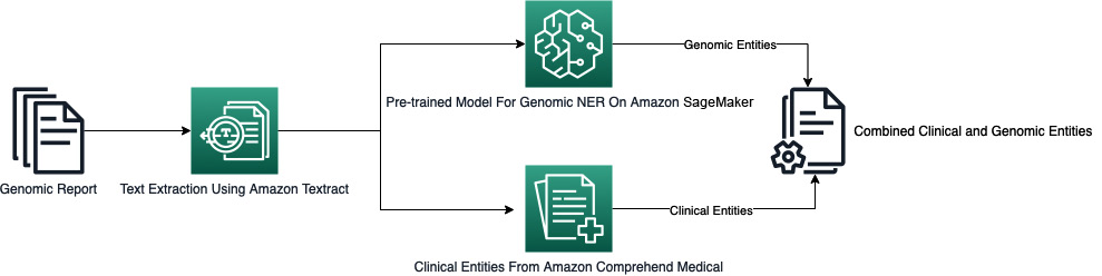
Figure 7.1 – Workflow for the NER application
The purpose of the application is to create an automated workflow to extract genetic and clinical entities from a genomic testing report. As shown in the preceding diagram, we will be using three key AWS services to build our application:
- Amazon Textract: We will use Textract to analyze the genomic testing report in PDF format and get the line-by-line text on each page of the report.
- Amazon SageMaker: We will use a SageMaker real-time model endpoint hosting a pre-trained model from the Hugging Face Model Hub to detect genetic entities from unstructured text. We will send lines of text from the genomic testing report to this model to detect genetic entities.
- Amazon Comprehend Medical: We will use Amazon Comprehend Medical to extract clinical entities from the same text in the report.
The final result will have all the genomic as well as clinical entities detected from the report. Before you begin, make sure you have access to SageMaker Studio and have set up Amazon Textract and S3 as described in the prerequisites section.
Acquiring the genomic test report
We will begin by downloading a sample test report from The Cancer Genome Atlas (TCGA) portal. This will be our source of the text on which we will run NER models.
Note
This exercise uses the Jupyter notebook that we downloaded in the Technical requirements section. The notebook has instructions and documentation about the steps in the exercise. Follow these steps to set up the notebook.
- To download the sample report, visit the following URL: https://portal.gdc.cancer.gov/repository?filters=%7B%22op%22%3A%22and%22%2C%22 content%22%3A%5B%7B%22op%22%3A%22in%22%2C%22content%22%3A%7B%22field%22%3A%22files.data_format%22%2C%22value%22%3A%5B%22pdf%22%5D%7D%7D%5D%7D.
The URL opens up the TCGA portal and applies the appropriate filters to show you a list of PDF reports. These are redacted pathology reports for breast cancer testing and consist of multiple pages.
- You can pick any report from this list to use in this application. To make it easy for you to follow along, let’s pick the file ER0197 ER-AC0F Clinical Report_Redacted_Sanitized.pdf. Click on the hyperlink for this file to open the download page. Click on the download link. There is a search field on the left where you can type ER0197 to help you find the file easily.
- Unzip/untar the downloaded file. This will create a folder with the name starting with gdc_download_. There will also be another folder within that whose name will look like a hash key. Inside this folder, you will see a PDF file. This is the source PDF file that we will use for our models.
Note
If you are using a Windows-based computer, you can use WinZip to untar the tar file. See more details can be found here: https://www.winzip.com/en/learn/file-formats/tar/.
- Open the PDF file and examine its contents. Once you are ready, upload the PDF file to the S3 bucket you created as part of the prerequisites.
You are now ready to run the notebook genetic_ner.ipynb to complete the exercise. However, before you do that, let us get a better understanding of the pre-trained model that we use in this exercise.
Understanding the pre-trained genetic entity detection model
As described earlier, we will be using a pre-trained NER model to detect genetic entities. The model we will use is available as a Hugging Face transformer. Hugging Face transformers provide an easy way to fine-tune and use pre-trained models for a variety of tasks involving text, tabular data, images, or multimodal datasets. Hugging Face maintains these models in a central repository known as the Hugging Face Hub. You can reference these models directly from the Hub and use them in your workflows. To learn more about Hugging Face transformers, you can visit the following link: https://huggingface.co/docs/transformers/index.
The model we will be using today is available on the Hugging Face Hub at the following link: https://huggingface.co/alvaroalon2/biobert_genetic_ner.
The model we will use is known as biobert_genetic_ner. The model is a fine-tuned version of the BioBERT model for NER tasks. It has been fine-tuned on certain datasets such as Bio Creative II Gene Mention Recognition (BC2GM). To learn more about the model, visit the Hugging Face Hub link: https://huggingface.co/alvaroalon2/biobert_genetic_ner.
Although not required to complete this exercise, it is also a good idea to familiarize yourself with transformer-based architecture for language understanding. It uses deep bidirectional transformers to understand unlabeled text and has achieved state-of-the-art performance on a variety of NLP tasks. You can learn more about it at the following link: https://arxiv.org/abs/1810.04805.
Once you are ready, open the notebook genetic_ner.ipynb in SageMaker Studio by navigating to Applied-Machine-Learning-for-Healthcare-and-Life-Sciences-using-AWS/chapter-7/. The notebook has instructions to complete the exercise. At the end of the exercise, you will see the output from the model that recognizes genomic and clinical entities from the test report. Here is a snapshot of what the output will look like:
- Her2neu
   Type: GENETIC
- immunoperoxidase panel
   Type: TEST_NAME
   Category: TEST_TREATMENT_PROCEDURE
- immunoperoxidase
   Type: GENETIC
- cleared
   Type: DX_NAME
   Category: MEDICAL_CONDITION
   Traits:
    - NEGATION
Let’s review what we’ve learned in this chapter.
Summary
In this chapter, we went into the basics of genomics. We defined key terminology related to genetics and understood how genomes influence our day-to-day functions. We also learned about genomic sequencing, the process of decoding genomic information from our DNA. We then learned about the challenges that organizations face when processing genomic data at scale and some techniques they can use to mitigate those challenges. Lastly, we learned about the inference options of SageMaker and hosted a pre-trained model on a SageMaker real-time endpoint. We combined this model with clinical entity recognition from Comprehend Medical to extract genetic and clinical entities from a genomic testing report.
In Chapter 8, Applying Machine Learning to Molecular Data, we will look at how ML is transforming the world of molecular property prediction. We will see how ML-based approaches are allowing scientists to discover unique drugs faster and with better outcomes for patients.
Further reading
- Understanding a genome: https://www.genome.gov/genetics-glossary/Genome
- DNA sequencing fact sheet: https://www.genome.gov/about-genomics/fact-sheets/DNA-Sequencing-Fact-Sheet
- Definition of DNA: https://www.britannica.com/science/DNA
- Next-Generation Sequencing: https://www.ncbi.nlm.nih.gov/pmc/articles/PMC3841808/
- Genomic data processing overview: https://gdc.cancer.gov/about-data/gdc-data-processing/genomic-data-processing