Every 3D model has a pivot point, also called its origin, which is the point around which the model will rotate and scale. In a 3D modeling package this point can be positioned wherever you want it to be, but to make the mathematics easier in a game we would normally treat the point (0, 0, 0) as the pivot point.

Each triangle in the model is defined by three vertices, and each vertex consists of an x, y, and z component which declares the position of the vertex in what is called model space (sometimes also referred to as object space). This just means that the components of each vertex are relative to the model's pivot point.

The following diagram shows an example of a cube. The pivot point is positioned at the very centre of the cube and is hence the origin of model space. The corner points use both positive and negative values, but each component has an absolute value of 100, which yields a cube with edges of length 200 units. For clarity, the three front faces of the cube also show how they have been built from two triangles.

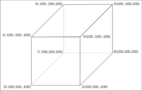
In order to provide Marmalade with the vertices of the cube, we simply use Marmalade's three-component floating pointer vector class CIwFVec3 to provide an array of vertices. As with the 2D rendering, we've already seen this is called a vertex stream, except that this time the stream consists of three component vectors.

You will notice that the corners of the cube in the previous diagram have been labeled with a number as well as their model space coordinates. If we cast our minds back to our work with 2D graphics, we will remember that Marmalade renders polygons by accepting a stream of vertices as input and also a stream of indices that defines the order in which those vertices should be processed.

The same approach applies when rendering 3D graphics. We specify the index stream as an array of unsigned 16-bit integers (uint16) and this dictates the order in which the vertices will be read out of the stream for rendering.

One advantage of using an index stream is that we can potentially refer to the same point several times without having to duplicate it in the vertex stream, thus saving us some memory. Since the index stream is just telling the GPU which order it has to process the data contained in the vertex, color, UV, and normal streams, it can be as long or as short as we want it to be. The index stream doesn't even need to reference every single element of the other streams, meaning we could potentially create one set of streams that can be referenced by multiple different index streams.

Another advantage of index streams is that we can use them to speed up rendering. You will recall that we used the function call IwGxDrawPrims to render a 2D polygon. To render 3D polygons, we use the exact same call. Each call to this function results in the rendering engine having to perform some initialization, so if we can find a way to minimize the number of draw calls we have to make, we can render the game world more quickly.

We can use the index stream to achieve this by inserting degenerate polygons into the polygon render list. A degenerate polygon is one that does not modify any pixels when it is drawn and this is achieved by ensuring that all the vertices that make up the polygon will lie on the same line. Most graphics hardware are clever enough to recognize a degenerate polygon and will not waste time trying to render it.

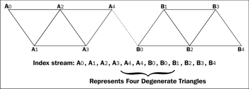
As an example, let's assume we are rendering some triangle strips. We could render them by calling IwGxDrawPrims twice, or we could join the two strips with some degenerate polygons and render them both with a single call to IwGxDrawPrims. We can continue to do this to join together as many triangle strips as we want.

How do we specify the degenerate triangle? The easiest way, shown in the following diagram, is to duplicate the last point of the first strip and the first point of the second strip. This yields four degenerate triangles (A3A4A4, A4A4B0, A4B0B0, B0B0B1) but is preferable to making several draw calls. The dotted line in the following diagram shows the extra degenerate triangles (which collapse to form a line!) that join the strips together:

Just as with 2D rendering, there are a number of other stream types we can supply to make the polygons we render look more interesting. We can provide both color and texture UV streams in exactly the same way we did when rendering in two dimensions, but we can also specify a third stream type called a normal stream.

In 3D mathematics, a normal vector is defined as the vector which is perpendicular to two other non-parallel vectors, or in other words a vector that points in the direction in which the polygon is facing. The following diagram shows an example illustrating this:

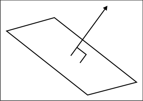
Why is the normal stream useful? Well, it allows us to simulate the effects of lights on our 3D model. By providing each vertex of our model with a unit normal (that is, a vector that points in the direction of the polygon's normal and which has a length of one unit), we can calculate the amount of light reflected from that vertex and adjust the color it is rendered with accordingly.

Real time lighting of a 3D model can be a time-intensive task, so when writing a game we try to avoid doing so when possible in order to speed up rendering. If we do not want to light a 3D model, there is no need to specify a normal stream; so, by not lighting a model we save memory too.

There are a couple of points to bear in mind when specifying these additional streams.

Firstly, Marmalade expects the number of colors, UVs, and normals provided to match the number of vertices provided. While you can specify streams of different lengths, this will normally cause an assert to be fired and obviously it could yield unexpected results when rendering.

Secondly, and perhaps most importantly, these additional streams may require us to add extra copies of our vertices into the vertex stream since we can only provide a single index stream.

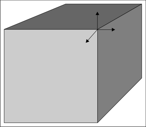
Take the example of a cube where each vertex is a corner point of three different faces of the cube. Since each face points in a different direction, we will need to duplicate each vertex three times so it can be referenced in the index stream along with the three different normal vectors.

We can also run into the same problem when the UV or color at a vertex varies across each polygon that it forms a part of.

For each different combination of color, UV, and normal we encounter, we need to provide an additional copy of each vertex, and therefore also an additional color, UV, and normal value so that all the streams are the same length.

Think back to school math lessons and you will hopefully remember matrices being described as a useful tool when trying to perform operations such as rotations, translations, and scaling on vectors.

My personal recollection about learning matrices was that they seemed slightly magical at the time. Here was a grid of numbers that could be used to perform a range of really useful geometric operations and, what's more, you could combine several matrices by multiplying them together to perform several operations in one go. The concept itself made sense, but there were so many numbers involved that it seemed a bit bewildering.

In 3D geometry we generally use a 4 x 4 matrix, with the top left 3 x 3 grid of numbers representing the rotation and scaling part of the matrix, and the first three numbers of the bottom row representing the required translation.

While the translation part made perfect sense to me, the 3 x 3 rotation and scaling part of the matrix was something I never really had a good handle on until the day I found out that what this part of the matrix actually represents is the size and direction of the x, y, and z axes.

Take a look at the following image that shows the identity matrix for a 4 x 4 matrix. All this means is that every element in the matrix is 0 except for those in the top-left to bottom-right diagonal, which are all 1:

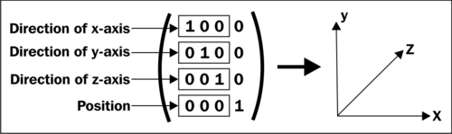
Notice that the first three numbers on the top row are (1, 0, 0), which just so happens to be a unit vector along the x axis. Similarly, the second row is (0, 1, 0), which represents a unit vector along the y axis and the third row (0, 0, 1) is a unit vector along the z axis.

Once I realized this, it became much more obvious how to create matrices to perform different kinds of geometric operations.

Want a rotation around the y axis? Just work out vectors for the directions in which the x axis and z axis would need to lie for the desired rotation, and slot these into the relevant parts of the matrix. Similarly, a scale operation just means that we provide a non-unit-sized vector for each axis we want to scale along.

Some of you may be reading this and thinking "that's obvious", but if this helps just one person to get a better understanding of how to understand matrix mathematics, my work is done!

When we looked at how a 3D model is represented in terms of data, we talked about the vertices of the model being in model space. In order to use these vertices for rendering, we therefore have to convert our model space vertices into screen coordinates.

The first step in this process is to use a model matrix to convert the vertices from model space into world space. Each vertex in the model is multiplied by the model matrix, which will first rotate and scale the vertices so that the model is orientated correctly, then translate each point so that the model's pivot point is now at the translation provided in the matrix.

Now that all our vertices are positioned correctly in our virtual world, the next step is to convert them into view space, which is the coordinate system defined by the position and orientation of our viewpoint, which for obvious reasons is normally referred to as our camera. We do this by providing another matrix called the view matrix (or camera matrix if you prefer), which will rotate, scale, and translate the world space vertices so that they are now relative to our camera view.

With the vertices now in view space, the final operation is to convert the vertices into 2D screen coordinates. We have two ways of doing this, these being an orthographic projection or a perspective projection.

An orthographic projection takes the view space coordinates and just scales and translates the x and y components of each vertex to put them onto the screen. The z component of the vertex plays no part in calculating the actual screen coordinates but it is used for working out the drawing order of polygons since it is used as a depth value.

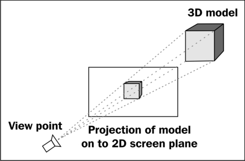
However, in most cases we use a perspective projection. Again the x and y components of each view space vertex are used to generate the x and y screen coordinates, but this time they are divided by the z component of the vertex, which has the effect of making objects that are further away appear smaller.

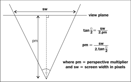
The components are also multiplied by a constant value called the perspective multiplier . This value is actually the distance at which the view plane lies from the camera. The view plane is the plane which contains the rectangular area of the screen display.

Normally, when we think about a camera view it is more convenient to think about the field of view, which is the horizontal angle of our viewing cone. The following diagram shows how we can convert this angle into the correct perspective multiplier value:

The next part of perspective projection is to translate the projected point. Normally we want a point that is directly in front of the camera to be in the center of the screen, so we would add an offset of half the screen width to the x component and half the screen height to the y-component. It is possible to specify a different offset position, which is particularly useful if we ever want to display a 3D model as part of a game's user interface. Let's say you wanted to draw a 3D model of a collectable object that the player has just picked up at the top right of the screen. Specifying the offset to be this screen position is much easier than trying to calculate a position in 3D space relative to the camera position that equates to the required area of the screen.

We've already discussed the view plane as being the plane which contains the final screen display, but there are some further planes which are used to help speed up rendering and also avoid some strange graphical glitches from occurring.

First we have the far clip plane and the near clip plane, which lie parallel to the view plane. We tell Marmalade where we want these planes to reside by supplying the perpendicular distance of these planes from the camera view point.

The far clip plane prevents polygons that are too far away from the camera from being rendered, while the near clip plane, unsurprisingly, prevents polygons that are too close to the camera from being rendered. The near clip plane is particularly important because if we were not to use it we would start to see models that lie behind the camera being rendered on screen.

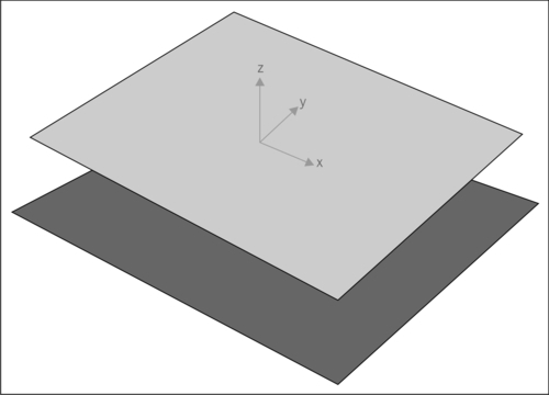
You should generally try to keep the far and near clip planes as close together as possible, as these values are also used for calculating depth buffer values. If the planes are too far apart, you can start to encounter render issues that are sometimes called shimmering or Z-fighting. These can occur when there is not enough resolution in the depth buffer values, which results in far distance polygons rendering with jagged edges or worse still, randomly poke through each other as they or the camera are moved. The following image shows another example of Z-fighting that can occur when trying to render two overlapping co-planar polygons:

There are also four more clipping planes named left, right, top, and bottom. These are planes which pass through the camera position and one of the left, right, top, or bottom borders of the screen display area on the view plane. Together they form a pyramid-shaped volume that emanates from the camera and defines the part of 3D space that is visible and could therefore appear on screen.

The clipping planes are managed automatically for us by Marmalade, and they are very useful as they allow us to quickly reject an entire model from being submitted for rendering if it is completely off screen. The off-screen check is performed using a bounding sphere for the model we are rendering, which is simply a sphere centered at the model's pivot point that encompasses all the vertices of the model. The bounding sphere can be quickly tested against all six clip planes and the model can be skipped if the bounding sphere is completely outside the clipping volume.

The simplest type of lighting Marmalade provides is emissive lighting, which is little more than the amount of color that a rendered polygon will naturally have. The emissive lighting color is provided by the CIwMaterial instance that is set when rendering the polygon.

Emissive lighting is useful if you want to draw polygons in a single flat color, but normally we want a bit more flexibility than that, so we might set a color stream instead, or use one of the other forms of lighting.

Ambient lighting provides the background level of light in our scene, such as the light which might be provided by the Sun.

Without ambient lighting, any polygon that is not facing a light source directly would have very little light applied to it and so would appear black. Normally this is not very desirable, so we can use ambient lighting to provide a base level of color and brightness to our polygons.

In Marmalade, we set a global ambient lighting term as an RGB color. The CIwMaterial instance used when rendering also has an ambient light value that is combined with the global ambient light. If the material ambient light is set to bright white, the polygon will be rendered with the full amount of the global ambient light.

If the global ambient lighting is disabled, the material ambient color is used directly to control the color of the rendered polygons. This provides an easy way of brightening or darkening a model at rendering time.

In order to use diffuse lighting our model data must provide a normal stream. A diffuse light comprises of both a color and a direction in which the light is pointing. The light's direction vector is combined with the normal vector for each vertex in the model using the dot product operation.

The result of the dot product operation is multiplied by the global diffuse lighting color and the current CIwMaterial diffuse color or the RGB value from the color stream, if one has been provided. This will yield the final color value that is used when rendering the polygon to the screen.

As with diffuse lighting, specular lighting can only work if we have provided a normal stream. It also needs a diffuse light to be specified as it relies on the direction of the diffuse light.

This type of lighting allows us to make a model appear shinier by causing it to briefly become brighter when it is facing the direction of the diffuse light.

We can specify both a global and a specular light color specific to CIwMaterial, and additionally the material also provides a setting for the specular power . This value allows us to narrow down the response of the specular lighting. A higher number means that the vertex normal must be almost parallel to the lighting direction before the specular lighting will take effect.